Dynamics of the Weil-Petersson flow: basic geometry of the Weil-Petersson metric I

Today we will define the Weil-Petersson (WP) metric on the cotangent bundle of the moduli spaces of curves and, after that, we will see that the WP metric satisfies the first three items of the ergodicity criterion of Burns-Masur-Wilkinson (stated as Theorem 3 in the previous post).

In particular, this will “reduce” the proof of the Burns-Masur-Wilkinson theorem (of ergodicity of WP flow) to the verification of the last three items of Burns-Masur-Wilkinson ergodicity criterion for the WP metric and the proof of the Burns-Masur-Wilkinson ergodicity criterion itself.

We organize this post as follows. In next section we will quickly review some basic features of the moduli spaces of curves. Then, in the subsequent section, we will start by recalling the relationship between quadratic differentials on Riemann surfaces and the cotangent bundle of the moduli spaces of curves. After that, we will introduce the Weil-Petersson and the Teichmüller metrics. Finally, the last section of this post will concern the verification of the first three items of the Burns-Masur-Wilkinson ergodicity criterion for the WP metric.

The basic reference for the next two sections is Hubbard’s book.

1. Moduli spaces of curves

1.1. Definition and examples of moduli spaces

Let be a fixed topological surface of genus with punctures. The moduli space is the set of Riemann surface structures on modulo biholomorphisms (conformal equivalences).

Example 1 (Moduli space of triply punctured spheres) The moduli space of triply punctured spheres consists of a single point

where denotes the Riemann sphere. Indeed, this is a consequence of the fact/exercise that the group of biholomorphisms (Möbius transformations) of the Riemann sphere is simply 3-transitive, i.e., given points , there exists an unique biholomorphism of sending , and (resp.) to , and (resp.).

Example 2 (Moduli space of once punctured torii) The moduli space of once punctured torii is

where the group acts on the hyperbolic half-plane via Möbius transformations (i.e., acts on via ). Indeed, this fact (previously explained in this post here) follows from the facts that a complex torus with a marked point is biholomorphic to a “normalized” lattice for some (with the marked point corresponding to the origin) and two “normalized” lattices are and are biholomorphic if and only if for some .

The second example reveals an interesting feature of : it is not a manifold, but only an orbifold. In fact, the stabilizer of the action of on at a typical point is trivial, but it has order at and order at (this corresponds to the fact that a typical torus has no symmetry, but the square and hexagonal torii have some symmetries). In particular, is topologically an once punctured sphere with two conical singularities at and . For a classical fundamental domain of the action of on , see the figure below (and also this one in the Wikipedia article on the modular group)

Moduli space of elliptic curves

As it turns out, all moduli spaces are complex orbifolds. In order to see this fact, we need to introduce some auxiliary structures (including the notions of Teichmüller spaces and mapping class groups).

Remark 1 From now on, we will restrict our attention to the case of a topological surface of genus with punctures such that . In this case, the uniformization theorem says that a Riemann surface structure on is conformally equivalent to a quotient of the hyperbolic upper-half plane by a discrete subgroup of (isomorphic to the fundamental group of ). Moreover, the hyperbolic metric on descends to a finite area hyperbolic metric on and, in fact, is the unique Riemannian metric of constant curvature on inducing the same conformal structure. (See, e.g., Hubbard’s book for more details)

1.2. Teichmüller metric

Let us start by endowing the moduli spaces with the structure of complete metric spaces.

By definition, a metric on corresponds to a way to “compare” (measure the distance) between two distinct points in the moduli space . A natural way of telling how far apart are two conformal structures on is by the means of quasiconformal maps.

Very roughly speaking, the idea is that even though by definition there is no conformal maps (biholomorphisms) between conformal structures and corresponding two distinct points of , one has several quasiconformal maps between them, that is, such that the quantity

is finite.

Here, it is worth to point out that is measuring the largest possible eccentricity among all infinitesimal ellipses in the tangent planes obtained as images under of infinitesimal circles on the tangent planes (see this post here or Hubbard’s book for more details [including some pictures of the geometrical meaning of ]), and, moreover, is conformal if and only if .

This motivates the following way of measuring the “distance” between and :

This function is the so-called Teichmüller metric (because, of course, it can be shown that is a metric on ).

The moduli space endowed with is a complete metric space.

Example 3 The Teichmüller metric on the moduli space of once-punctured torii can be shown to coincide with the hyperbolic metric induced by Poincarés metric on (see Hubbard’s book).

1.3. Teichmüller spaces and mapping class groups

Once we know that the moduli spaces are topological spaces (and, actually, complete metric spaces), we can start the discussion of its universal cover.

In this direction, we need to describe the “fiber” in the universal cover of a point of (i.e., a complex (Riemann surface) structure on ). In other terms, we need to add “extra information” to . As it turns out, this “extra information” has topological nature and it is called a marking.

More precisely, a marked complex structure (on ) is the data of a Riemann surface together with a homeomorphism (called marking).

By analogy with the notion of moduli spaces, we define the Teichmüller space is the set of Teichmüller equivalence classes of marked complex structures, where two marked complex structures and are Teichmüller equivalent whenever there exists a conformal map isotopic to . In other words, the Teichmüller space is the “moduli space of marked complex structures”.

The Teichmüller metric also makes sense on the Teichmüller space and the metric space is also complete.

From the definitions, we see that one can recover the moduli space from the Teichmüller space by forgetting the “extra information” given by the markings. Equivalently, we have that where is the so-called mapping class group of isotopy classes of orientation-preserving homeomorphisms of .

The mapping class group is a discrete group acting on by isometries of the Teichmüller metric . Moreover, by Hurwitz theorem (and the fact that we are assuming that ), the -stabilizer of any point of is finite (of cardinality when ), but it might vary from point to point because some Riemann surfaces are more symmetric than others (see, e.g., Example 2 above).

Example 4 The Teichmüller space of once-punctured torii is . Indeed, the set of once-punctured torii is parametrized by normalized lattices , , and there is a conformal map between and if and only if , . Now, using this information one can check that and (because the conformal map associated to is isotopic to the identity if and only if ).

The Teichmüller space is the universal cover of and is the (orbifold) fundamental group of (compare with the example above). A common way to see this fact passes through showing that is simply connected (and even contractible) because it admits a global system of coordinates called Fenchel-Nielsen coordinates (providing an homemorphism between and ). The discussion of these coordinates is the topic of the next subsection.

1.4. Fenchel-Nielsen coordinates

In order to introduce the Fenchel-Nielsen coordinates, we need the notion of pants decomposition. A pants (trouser) decomposition of is a collection of simple closed curves on that are pairwise disjoint, homotopically non-trivial (i.e., not homotopic to a point) and non-peripheral (i.e., not homotopic to a small loop around one of the possible punctures of ). The picture below illustrates a pants decomposition of a compact surface of genus :

The nomenclature “pants decomposition” comes from the fact that if we cut along the curves , (i.e., we consider the connected components of the complement of these curves), then we see “pairs of pants” (topologically equivalent to a triply punctured sphere):

A remarkable fact about pair of pants/trousers is that hyperbolic/conformal structures on them are uniquely determined by the (hyperbolic) lengths of their boundary components. In other terms, a trouser with boundary circles ( or ) has a -dimensional space of hyperbolic structures (parametrized by the lenghts of these -circles). Alternatively, one can construct trousers out of right-angled hexagons in the hyperbolic plane (see, e.g., Theorem 3.5.8 in Hubbard’s book).

In this setting, the Fenchel-Nielsen coordinates can be described as follows. We fix a pants decomposition and we consider

defined by , where is the hyperbolic length of with respect to the hyperbolic structure associated to the marked complex structure , and is a twist parameter measuring the “relative displacement” of the pairs of pants glued at .

A detailed description of the twist parameters can be found in Section 7.6 of Hubbard’s book, but, for now, let us just make some quick comments about them. Firstly, we fix (in an arbitrary way) a collection of simple arcs joining the boundaries of the pairs of pants determined by such that these arcs land at the same point whenever they come from opposite sides of .

From these arcs, we get a collection of simple closed curves on looking like this:

Consider now a pair of trousers sharing a curve (they might be the same trouser) and let be an arc of a curve in joining two boundary components and of the union of these trousers:

Given a marked complex structure , consider the unique arc on homotopic to (relative to the boundary of the union of the pair of trousers) consisting of two minimal geodesic arcs connecting to and and an immersed geodesic moving inside . We define the twist parameter as the oriented length of counted as positive if it turns to the right and negative if it turns to the left. The figure below illustrates two markings and whose twist parameters differ by

Remark 2 The fact that the definition of the twist parameters depend on the choice of implies that the twist parameters are well-defined only up to a constant. Nevertheless, this technical difficulty does not lead to any serious issue.

In any case, it is possible to show the Fenchel-Nielsen coordinates associated to any pants decomposition is a global homeomorphism (see, e.g., Theorem 7.6.3 in Hubbard’s book). In particular, the Teichmüller space is simply connected (as it is homeomorphic to ). Hence, it is the universal cover of the moduli space (and the mapping class group is the orbifold fundamental group of ).

This partly explain why one discusses the properties of and at the same time.

2. Cotangent bundle of moduli spaces

Another reason for studying and together is because is a manifold while is only an orbifold. In fact, the Teichmüller spaces are real-analytic manifolds. Indeed, the real-analytic structure on comes from the uniformization theorem. More precisely, given a marked complex structure , we can apply the uniformization theorem to write where is a discrete subgroup isomorphic to the fundamental group of . In other words, from a marked complex structure , we have a representation of on (well-defined modulo conjugation), and this permits to identify with an open component of the character variety of homomorphisms from to modulo conjugacy. In particular, the pullback of the real-analytic structure of this representation variety to endow with its own real-analytic structure.

Actually, as it turns out, this real-analytic structure of can be “upgraded” to a complex-analytic structure. One way of seeing this uses a “generalization” of the construction of the real-analytic structure above based on the complex-analytic structure on the representation variety of in and Bers simultaneous uniformization theorem.

Remark 3 It is worth to compare this with the following “toy model” situation.Let be a real vector space of dimension and denote by the set of linear complex structures on (i.e., -linear maps with ). It is possible to check that a linear complex structure on is equivalent to the data of a complex subspace of the complexification of such that and (i.e., ) where is the complex conjugate of .

Since the condition is open in the Grassmanian manifold of complex subspaces of of complex dimension , and is naturally a complex manifold, we obtain that the set parametrizing complex structures on is itself a complex manifold.

We will discuss this point later (in a future post) and, for now, let us just sketch the relationship between the quadratic differentials on Riemann surfaces and the cotangent bundle to Teichmüller and moduli spaces (referring to this previous post for more details).

2.1. Integrable quadratic differentials

The Teichmüller metric was defined via the notion of quasiconformal mappings . By inspecting the nature of this notion, we see that the quantities (related to the eccentricities of infinitesimal ellipses obtained as the images under of infinitesimal circles) play an important role in the definition of the Teichmüller distance between and .

The measurable Riemann mapping theorem of Alhfors and Bers (see, e.g., page 149 of Hubbard’s book) says that the quasiconformal map can be recovered from the quantities up to composition with conformal maps. More precisely, by collecting the quantities in a globally defined tensor of type

with called Beltrami differential, one can “recover” by solving Beltrami’s equation

in the sense that there is always a solution to ths equation and, furthermore, two solutions and differ by a conformal map (i.e., ).

In other terms, the deformations of complex structures are intimately related to Beltrami differentials and it is not surprising that Beltrami differentials can be used to describe the tangent bundle of . In this setting, we can obtain the cotangent bundle by noticing that there is a natural pairing between bounded () Beltrami differentials and integrable () quadratic differentials (i.e., a tensor of type , ):

because is an area form and is integrable. In this way, it can be shown that the cotangent space at a point of is naturally identified to the space of integrable quadratic differentials on .

Note that the space of integrable quadratic differentials provides a concrete way of manipulating the complex structure of : in this setting, the complex structure is just the multiplication by on the space of quadratic differentials.

Remark 4 By a theorem of Royden (see Hubbard’s book), the mapping class group is the group of complex-analytic automorphisms of . In particular, the moduli space is a complex orbifold.

2.2. Teichmüller and Weil-Petersson metrics

Using the description of the cotangent bundle of in terms of quadratic differentials, we are ready to define the Teichmüller and Weil-Petersson metrics.

Given a point of , we endow the cotangent space with the -norm:

where is the hyperbolic metric associated to the conformal structure and is a quadratic differential (i.e., a tensor of type ).

Remark 5 More generally, we define the -norm of a tensor of type (i.e., ) as:

In this notation, the infinitesimal Teichmüller metric is the family of -norms on the fibers of the cotangent bundle of . Here, the nomenclature “infinitesimal Teichmüller metric” is justified by the fact that the “global” Teichmüller metric (defined by the infimum of the eccentricity factors of quasiconformal maps ) is the Finsler metric induced by the “infinitesimal” Teichmüller metric (see, e.g., Theorem 6.6.5 of Hubbard’s book).

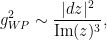
In a similar vein, the Weil-Petersson (WP) metric is the family of -norms on the fibers of the cotangent bundle of .

Remark 6 In the definition of the Weil-Petersson metric, it was implicit that an integrable quadratic differential has finite -norm (and, actually, all -norms are finite, ). This fact is obvious when the is compact, but it requires a (simple) computation when has punctures. See, e.g., Proposition 5.4.3 of Hubbard’s book for the details.

For later use, we will denote the (infinitesimal) Teichmüller metric, resp., Weil-Petersson metric, as , resp. .

The Teichmüller metric is a Finsler metric in the sense that the family of -norms on the fibers of vary in a but not way (cf. Lemma 7.4.3 and Proposition 7.4.4 in Hubbard’s book).

Remark 7 The first derivative of the Teichmüller metric is not hard to compute. Given two cotangent vectors with , we affirm that

Indeed, the first derivative is . Since and is bounded (i.e., its norm is finite), we can use the dominated convergence theorem to obtain that

The Weil-Petersson metric is induced by the Hermitian inner product

As usual, the real part induces a real inner product (also inducing the Weil-Petersson metric), while the imaginary part induces an anti-symmetric bilinear form, i.e., a symplectic form.

By definition, the Weil-Petersson metric relates to the Weil-Petersson symplectic form and the complex structure on (i.e., multiplication by of elements of ) via:

Furthermore, as it was firstly discovered by Weil by means of a “simple-minded calculation” (“calcul idiot”) and later confirmed by others, it is possible to show that the Weil-Petersson metric is Kähler, i.e., the Weil-Petersson symplectic form is closed (that is, its exterior derivative vanishes: ). See, e.g., Section 7.7 of Hubbard’s book for more details.

We will come back later (in a future post) to the Kähler property of the Weil-Petersson metric, but for now let us just mention that this property enters into the proof of a beautiful theorem of Wolpert saying that the Weil-Petersson symplectic form has a simple expression in terms of Fenchel-Nielsen coordinates:

where is an arbitrary pants decomposition of . Here, it is worth to mention that an important step in the proof of this formula (cf. Step 2 in the proof of Theorem 7.8.1 in Hubbard’s book) is the fact discovered by Wolpert that the infinitesimal generator of the Dehn twist about is of the symplectic gradient of the Hamiltonian function , that is,

This equation is the starting point of several Wolpert’s expansion formulas for the Weil-Petersson metric that we will discuss later in this series of posts.

Before proceeding further, let us briefly discuss the Teichmüller and Weil-Petersson metrics on the moduli spaces of once-punctured torii .

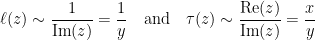
Example 5 The Teichmüller metric on is the quotient of the hyperbolic metric of .On the other hand, the Fenchel-Nielsen coordinates on have first-order expansion

where . Thus, we see from Wolpert’s formula that

Since the complex structure on is the standard complex structure of , we see that the Weil-Petersson metric has asymptotic expansion

that is, the Weil-Petersson on the moduli space near the cusp at infinity is modeled by the surface of revolution obtained by rotating the curve (for say). See the picture below. This is in contrast with the fact that the Teichmüller metric is the hyperbolic metric and hence it is modeled by surface of revolution obtained by rotation the curve (for say). (Recall that, in general, a surface of revolution obtained by rotation of the curve has the metric ) From this asymptotic expansion of , we see that it is incomplete: indeed, a vertical ray to the cusp at infinity starting at a point in the line has Weil-Petersson length . Moreover, the curvature satisfies , and, in particular, as .

The previous example (Weil-Petersson metric on ) already contains several features of the Weil-Petersson metric on general Teichmüller spaces and moduli spaces .

In fact, we will see later that the Weil-Petersson metric is incomplete because it is possible to shrink a simple closed curve to a point and leave Teichmüller space along a Weil-Petersson geodesic in time . Also, some sectional curvatures might approach as one leaves Teichmüller space.

Nevertheless, an interesting feature of the Weil-Petersson metric in and for not occuring in the case of is the fact that some sectional curvatures might also approach as one leaves Teichmüller space. Indeed, as we will see later, this happens because the “boundary” of is sufficiently “large” when so that it is possible form some Weil-Petersson geodesics to travel “almost parallel” to certain parts of the “boundary” for a certain time (while the same is not possible for because the “boundary” consists of a single point).

After this brief introduction of our main dynamical object (Weil-Petersson geodesic flow), we can now start the discussion of the proof of Burns-Masur-Wilkinson theorem (on the ergodicity of the Weil-Petersson flow). The basic reference for the next two sections is Burns-Masur-Wilkinson paper.

3. Burns-Masur-Wilkinson theorem and ergodicity of the Weil-Petersson flow on finite covers of moduli spaces

Recall that the statement of Burns-Masur-Wilkinson ergodicity criterion for geodesic flows on manifolds is:

Theorem 1 (Burns-Masur-Wilkinson) Let be the quotient of a contractible, negatively curved, possibly incomplete, Riemannian manifold by a subgroup of isometries of acting freely and properly discontinuously. Denote by the metric completion of and the boundary of .Suppose that:

• (I) the universal cover of is geodesically convex, i.e., for every , there exists an unique geodesic segment in connecting and .
• (II) the metric completion of is compact.
• (III) the boundary is volumetrically cusplike, i.e., for some constants and , the volume of a -neighborhood of the boundary satisfies

  

  for every .

• (IV) has polynomially controlled curvature, i.e., there are constants and such that the curvature tensor of and its first two derivatives satisfy the following polynomial bound

  

  for every .

• (V) has polynomially controlled injectivity radius, i.e., there are constants and such that

  

  for every (where denotes the injectivity radius at ).

• (VI) The first derivative of the geodesic flow is polynomially controlled, i.e., there are constants and such that, for every infinite geodesic on and every :

  

Then, the Liouville (volume) measure of is finite, the geodesic flow on the unit cotangent bundle of is defined at -almost every point for all time , and the geodesic flow is non-uniformly hyperbolic (in the sense of Pesin’s theory) and ergodic.

Actually, the geodesic flow is Bernoulli and, furthermore, its metric entropy is positive, finite and is given by Pesin’s entropy formula (i.e., it is equal to the sum of positive Lyapunov exponents of counted with multiplicities).

The goal of this section is to show how the ergodicity criterion above can be used to deduce the following theorem (Burns-Masur-Wilkinson theorem on the ergodicity of the Weil-Petersson geodesic flow).

Theorem 2 (Burns-Masur-Wilkinson) The Weil-Petersson flow on the unit cotangent bundle of is ergodic (for any , ) with respect to the Liouville measure of the WP metric. Actually, it is Bernoulli (i.e., it is measurably isomorphic to a Bernoulli shift) and, a fortiori, mixing. Furthermore, its metric entropy is positive and finite.

At first sight, it is tempting to say that Theorem 2 follows from Theorem 1 after checking items (I) to (VI) for the case (the cotangent bundle of ), (the cotangent bundle of ) and (the mapping class group).

However, this is not quite true because the moduli spaces and their unit cotangent bundles are not manifolds but only orbifolds, while we assumed in Theorem 1 that the phase space of the geodesic flow is a manifold.

In other words, the orbifoldic nature of moduli spaces imposes a technical difficulty in the reduction of Theorem 2 to Theorem 1. Fortunately, a solution to this technical issue is very well-known to algebraic geometers and it consists into taking an adequate finite cover of the moduli space in order to “kill” the orbifold points (i.e., points with large stabilizers for the mapping class group).

More precisely, for each , one considers the following finite-index subgroup of the mapping class group :

where is the action on homology of . Equivalently, an element of belongs to whenever its action on the absolute homology group corresponds to a (symplectic) integral matrix congruent to the identity matrix modulo .

Example 6 In the case of once-punctured torii, the mapping class group is and

In the literature, is called the principal congruence subgroup of of level .

Remark 8 The index of in can be computed explicitly. For instance, the natural map from to is surjective (see, e.g., Farb-Margalit’s book), so that the index of is the cardinality of , and, for prime, one has

cf. Dickson’s book.

It was shown by Serre (see the appendix of this paper here for the original proof and the Chapter 6 of the book of Farb-Margalit for an alternative exposition) that is torsion-free for and, a fortiori, it acts freely and properly discontinuous on for . In other terms, the finite cover of given by

is a manifold for .

Remark 9 Serre’s result is sharp: the principal congruence subgroup of level of contains the torsion element .

Once one disposes of an appropriate manifold finitely covering the moduli space , the reduction of Theorem 2 to Theorem 1 consists into two steps:

• (a) the verification of items (I) to (VI) in the statement of Theorem 1 in the case of the unit cotangent bundle of .
• (b) the deduction of the ergodicity (and mixing, Bernoullicity, and positivity and finiteness of metric entropy) of the Weil-Petersson geodesic flow on from the corresponding fact(s) for the Weil-Petersson geodesic flow on .

For the remainder of this section, we will discuss item (b) while leaving the first part of item (a) (i.e., items (I), (II) and (III) of Theorem 1 for ) for the next section and the second part of item (a) (i.e., items (I), (II) and (III) of Theorem 1 for )) for the next post.

For ease of notation, we will denote , and . Assuming that the Weil-Petersson flow is ergodic (and Bernoulli, and its metric entropy is positive and finite) on , the “obstruction” to show the same fact(s) for the Weil-Petersson flow on is the possibility that the orbifold points of form a “large” set.

Indeed, if we can show that the set of orbifold points of is “small” (e.g., they form a set of zero measure), then the geodesic flow on covers the geodesic flow on on a set of full measure. In particular, if is a (Weil-Petersson flow) invariant set of positive measure on , then its lift to is also a (Weil-Petersson flow) invariant set of positive measure. Therefore, by the ergodicity of the Weil-Petersson flow on , we have that has full measure, and, a fortiori, has full measure. Moreover, the fact that the Weil-Petersson flow on covers the Weil-Petersson flow on on a full measure set also allows to deduce Bernoullicity and positivity and finiteness of metric entropy of the latter flow from the corresponding properties for the former flow.

At this point, it remains only to check that the orbifold points of for a subset of zero measure (for the Liouville/volume measure of the Weil-Petersson metric) in order to complete the discussion of this section. In this direction, we have that the following fact:

Lemma 3 Let be the subset of corresponding to orbifoldic points, i.e., is the (countable) union of the subsets of fixed points of the natural action on of all elements of finite order, excluding the genus hyperelliptic involution. Then, is a closed subset of real codimension (at least).

Proof: For each of finite order, is the Teichmüller space of the quotient orbifold . From this, one can show that:

• if is compact and is not the hyperelliptic involution in genus , then has complex dimension ;
• if has punctures, then has complex dimension ;
• if is the hyperelliptic involution in genus , then .

See, e.g., this paper of Rauch for more details.

In particular, the proof of the lemma is complete once we verify that is a locally finite union of the real codimension subsets , .

Keeping this goal in mind, we fix a compact subset of and we recall that the mapping class group acts in a properly discontinuous manner on . Therefore, it is not possible for an infinite sequence of distinct finite order elements to satisfy for all . In other words, is the subset of finitely many , i.e., is a locally finite union of , .

Example 7 In the case of once-punctured torii, the subset consists of the -orbits of the points and .

4. Geometry of the Weil-Petersson metric: part I

In this section, we will discuss three properties of the Weil-Petersson metric on and related to the items (I), (II) and (III) in the statement of Theorem 1 above.

We start by noticing that the item (I) in the statement of Theorem 1 (i.e., the geodesic convexity of the Weil-Petersson metric on ) was proved by Wolpert in this paper here.

Next, the fact that it is possible to leave the Teichmüller space along a Weil-Petersson geodesic in finite time of order was exploited by Masur to show that the metric completion of the (equipped with the Weil-Petersson metric) is the so-called augmented Teichmüller space . As it turns out, the mapping class group acts on and the quotient

is the so-called Deligne-Mumford compactification of the moduli space (giving the metric completion of equipped with the Weil-Petersson metric).

The augmented Teichmüller space is a stratified space obtained by adjoining lower-dimensional Teichmüller spaces of noded Riemann surfaces. The combinatorial structure of the stratification of is encoded by the curve complex (also called complex of curves or graph of curves in the literature).

More precisely, the curve complex is a –simplicial complex defined as follows. The vertices of are homotopy classes of homotopically non-trivial, non-peripheral, simple closed curves on . We put an edge between two vertices whenever the corresponding homotopy classes have disjoint representatives. In general, a -simplex consists of distinct vertices possessing mutually disjoint representatives.

Remark 10 is a -simplicial complex because a maximal collection of distinct vertices possessing disjoint representatives is a pants decomposition of and, hence, .

Example 8 In the case of once-punctured torii, the curve complex consists of an infinite discrete set of vertices (because there is no pair of disjoint homotopically distinct curves). However, some authors define the curve complex of once-punctured torii by putting an edge between vertices corresponding to curves intersecting minimally (i.e., only once). In this definition, the curve complex of once-punctured torii becomes the Farey graph.

The curve complex is a connected locally infinite complex, except for the cases of the four-times punctured spheres and the once-punctured torii. Also, the mapping class group acts on . Moreover, Masur and Minsky showed that is -hyperbolic metric space for some .

Using the curve complex , we can define the augmented Teichmüller space as follows.

A noded Riemann surface is a compact topological surface equipped with the structure of a complex space with at most isolated singularities called nodes such that each of these singularities possess a neighborhood biholomorphic to a neighborhood of in the singular curve

Removing the nodes of a noded Riemann surface yields to a possibly disconnected Riemann surface denoted by . The connected components of are called the pieces of . For example, the noded Riemann surface of genus of the figure above has two pieces (of genera and 1 resp.).

Given a simplex , we will adjoint a Teichmüller space to in the following way. A marked noded Riemann surface with nodes at is a noded Riemann surface equipped with a continuous map such that the restriction of to is a homeomorphism to . We say that two marked noded Riemann surfaces and are Teichmüller equivalent if there exists a biholomorphic node-preserving map such that is isotopic to . The Teichmüller space associated to is the set of Teichmüller equivalence classes marked noded Riemann surfaces with nodes at .

In this context, the augmented Teichmüller space is

The topology on is given by the following neighborhoods of points . Given , we consider a maximal simplex (pants decomposition of ) containing and we let be the corresponding Fenchel-Nielsen coordinates on . We extend these coordinates by allowing whenever is pinched in a node and we take the quotient by identifying noded Riemann surfaces corresponding to parameters and whenever .

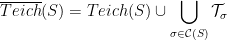
Remark 11 The augmented Teichmüller space is not locally compact: indeed, a neighborhood of a noded Riemann surface allows for arbitrary twists corresponding to curves .

The quotient of by the natural action of (through the corresponding action on ) is called Deligne-Mumford compactification of the moduli space (see, e.g., this paper of Hubbard and Koch for more details). Since is a finite-index subgroup of and is the metric completion of with respect to the Weil-Petersson metric, it follows that the the metric completion of with respect to the Weil-Petersson metric is also compact.

In particular, satisfies the item (II) in the statement of Theorem 1.

Remark 12 It is worth to notice that the Deligne-Mumford compactification in the case of the once-punctured torii is just one point (because geometrically by pinching one curve in a punctured torus we get a thrice-puncture sphere in the lmit) while it is stratified in non-trivial lower-dimensional moduli spaces in general. Moreover, as we will see later, some asymptotic formulas of Wolpert tells that the Weil-Petersson metric “looks” like a product of the Weil-Petersson metrics on these lower-dimensional moduli spaces. In particular, as we will discuss in the last post of this series, it will be possible for several Weil-Petersson geodesics to travel “almost parallel” to these lower-dimensional moduli spaces and this will give a polynomial rate of mixing for this flow in general. On the other hand, since it is not possible to travel almost parallel to a point for a long time, this arguments breaks down in the case of the Weil-Petersson metric in the case of the moduli space of once-punctured torii.

Finally, let us complete the discussion in this section by quickly checking that also satisfies the item (III) in the statement of Theorem 1, i.e., its boundary is volumetrically cusp-like.

In this direction, given , let us denote by the Weil-Petersson distance between and . Our current task is to prove that there are constants and such that

where .

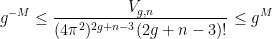
As we are going to see now, one can actually take in the estimate above thanks to some asymptotic formulas of Wolpert for the Weil-Petersson metric near .

Lemma 4 One has .

Proof: It was shown by Wolpert (in page 284 of this paper here) that the Weil-Petersson metric has asymptotic expansion

near , where and , are the Fenchel-Nielsen coordinates associated to .

This gives that the volume element of the Weil-Petersson metric near is . Furthermore, this also says that the distance between and is comparable to . By putting these two facts together, we see that

This proves the lemma.

Remark 13 Using the properties that the metric completion of is compact and is volumetrically cusp-like imply that the Liouville measure (volume) is finite.In a recent work, Mirzakhani studied the total mass of with respect to the Weil-Petersson metric and she showed that there exists a constant such that