Furstenberg’s theorem on the Poisson boundaries of lattices of SL(n,R) (part I)

Posted by: matheuscmss | July 21, 2013

Furstenberg’s theorem on the Poisson boundaries of lattices of SL(n,R) (part I)

In this previous blog post here (about this preprint joint with Alex Eskin), it was mentioned that the simplicity of Lyapunov exponents of the Kontsevich-Zorich cocycle over Teichmüller curves in moduli spaces of Abelian differentials (translation surfaces) can be determined by looking at the group of matrices coming from the associated monodromy representation thanks to a profound theorem of H. Furstenberg on the so-called Poisson boundary of certain homogenous spaces.

In particular, this meant that, in the case of Teichmüller curves, the study of Lyapunov exponents can be performed without the construction of any particular coding (combinatorial model) of the geodesic flow, a technical difficulty occurred in previous papers dedicated to the simplicity of Lyapunov exponents of the Kontsevich-Zorich cocycle (such as these articles here and here).

Of course, I was happy to use Furstenberg’s result as a black-box by the time Alex Eskin and I were writing our preprint, but I must confess that I was always curious to understand how Furstenberg’s theorem works. In fact, my curiosity grew even more when I discovered that Furstenberg wrote a survey article (of 63 pages) on this subject, but, nevertheless, this survey was not easily accessible on the internet. For this reason, after consulting a copy of Furstenberg’s survey at Institut Henri Poincaré (IHP) library, I was impressed by the high quality of the material (as expected) and I decided to buy the book containing this survey.

As the reader can imagine, I learned several theorems by reading Furstenberg’s survey and, for this reason, I thought that it could be a good idea to describe here the proof of a particular case of Furstenberg’s theorem on the Poisson boundary of lattices of ${SL(n,\mathbb{R})}$ (mostly for my own benefit, but also because Furstenberg’s survey is not easy to find online to the best of my knowledge).

For the sake of exposition, I will divide the discussion of Furstenberg’s survey into two posts, using Furstenberg’s survey, his original articles and A. Furman’s survey as basic references.

For this first (introductory) post, we will discuss (below the fold) some of the motivations behind Furstenberg’s investigation of Poisson boundaries of lattices of Lie groups and we will construct such boundaries for arbitrary (locally compact) groups equipped with probability measures.

1. Some Motivations

Definition 1 A lattice ${\Gamma}$ of a Lie group ${G}$ is a discrete subgroup such that the quotient ${G/\Gamma}$ has finite volume with respect to the natural invariant measure induced from the (left-invariant) Haar measure on ${G}$ .

Example 1 Among the most basic examples of lattices, one has: ${\Gamma_0=\mathbb{Z}^n}$ is a lattice of ${G_0=\mathbb{R}^n}$ , and ${\Gamma_1=SL(n,\mathbb{Z})}$ is a lattice of ${G_1=SL(n,\mathbb{R})}$ (cf. Zimmer’s book for instance).

Definition 2 We say that a non-compact Lie group ${G}$ is an envelope of ${\Gamma}$ whenever ${\Gamma}$ is isomorphic to a lattice of ${G}$ .

Example 2 The Lie group ${SL(2,\mathbb{R})}$ is an envelope of the free group on two generators ${F_2}$ . Indeed, it is possible to show that ${F_2=\langle A, B\rangle}$ is isomorphic to the level two congruence subgroup of ${SL(2,\mathbb{Z})}$

$\displaystyle \Gamma(2)=\left\{\left(\begin{array}{cc}a & b \\ c & d \end{array}\right)\in SL(2,\mathbb{Z}): a\equiv d\equiv 1, b\equiv c\equiv 0 (\textrm{mod }2)\right\}$

via the isomorphism ${A\mapsto \left(\begin{array}{cc}1 & 2 \\ 0 & 1 \end{array}\right)}$ and ${B\mapsto \left(\begin{array}{cc}1 & 0 \\ 2 & 1 \end{array}\right)}$ . Since ${\Gamma(2)}$ is a finite-index (actually index ${6}$ , cf. Bergeron’s book for example) subgroup of ${SL(2,\mathbb{Z})}$ (a lattice of ${SL(2,\mathbb{R})}$ , cf. Example 1), this shows that ${SL(2,\mathbb{R})}$ envelopes ${F_2}$ .

Example 3 The Lie group ${PSL(2,\mathbb{R}):=SL(2,\mathbb{R})/\{\pm Id\}}$ envelopes the fundamental group ${\pi_1(S)}$ of any compact surface of genus ${g\geq 2}$ . In fact, by fixing any Riemann surface structure on ${S}$ , we obtain from the uniformization theorem that ${S=\mathbb{H}^2/\Gamma}$ where ${\Gamma\simeq\pi_1(S)}$ is a subgroup of the group ${PSL(2,\mathbb{R})}$ of hyperbolic isometries (Möbius transformations) of the hyperbolic plane ${\mathbb{H}^2}$ . Note that ${\Gamma}$ is a lattice of ${PSL(2,\mathbb{R})}$ because ${PSL(2,\mathbb{R})/\Gamma}$ is naturally identified to the unit cotangent bundle of the compact surface ${S=\mathbb{H}^2/\Gamma}$ , so that, by definition, ${PSL(2,\mathbb{R})}$ envelopes ${\pi_1(S)}$ .

Once we have the notion of envelope ${G}$ of a (discrete) group ${\Gamma}$ , the following three questions arise naturally:

i) Existence: What are the (discrete) groups admitting envelopes?
ii) Uniqueness: If ${\Gamma}$ admits an envelope ${G}$ , to what extend is ${G}$ unique?
iii) Rigidity: Let ${\Gamma_1}$ and ${\Gamma_2}$ (resp.) be (discrete) groups enveloped by ${G_1}$ and ${G_2}$ (resp.) and assume that ${\Gamma_1}$ is isomorphic to ${\Gamma_2}$ , say via an isomorphism ${\iota:\Gamma_1\rightarrow\Gamma_2}$ . Is it true that this isomorphism ${\iota}$ is the restriction of an isomorphism ${\overline{\iota}: G_1\rightarrow G_2}$ of the Lie groups ${G_1}$ and ${G_2}$ ?

Here are some partial answers to these questions.

Firstly, all these questions have affirmative answers in the context of finitely generated nilpotent groups: see these references here for more details.

On the other hand, we do not dispose of complete answers in the other settings.

For instance, the existence question i) is open in general, but if we ask what discrete groups have semi-simple envelopes, then some necessary conditions are known. For example, H. Kesten proved in 1959 (see this paper here) that if ${\Gamma}$ is a finitely generated group, say that ${\Gamma}$ is generated by ${\gamma_1,\dots,\gamma_r}$ , and a semi-simple Lie group envelopes ${\Gamma}$ , then

$\displaystyle \lim\limits_{n\rightarrow\infty}\log(H_n)/n>0$

where ${H_n}$ is the number of elements of ${\Gamma}$ obtained as the products of at most ${n}$ of the ${g_i}$ ‘s and their inverses (i.e., elements of the form ${g_{i_1}^{\varepsilon_{i_1}}\dots g_{i_m}^{\varepsilon_{i_m}}}$ where ${\varepsilon_{i_j}=\pm1}$ for each ${j=1,\dots, m}$ and ${m\leq n}$ ).

Remark 1 Note that Kesten’s condition (of exponential growth of ${H_n}$ ) is independent of the particular set ${\{g_1,\dots,g_r\}}$ of generators of ${\Gamma}$ used. Moreover, it is not satisfied by Abelian groups and it is satisfied by free groups ${F_r}$ (on any number ${r\geq 2}$ of generators).

Also, the uniqueness question ii) is trivially false if we insist on a “simple-minded uniqueness”: indeed, from the definition, if ${G}$ is an envelope of ${\Gamma}$ , then ${G\times K}$ is also an envelope of ${\Gamma}$ whenever ${K}$ is a compact Lie group.

So, the uniqueness question ii) has some chance of having an affirmative answer only if we ask for uniqueness of the envelope modulo compact factors. In particular, it is natural to ask whether two Lie groups ${G_1}$ and ${G_2}$ without compact factors (i.e., for ${i=1, 2}$ , one has that ${G_i\not\simeq G_i'\times K_i}$ with ${K_i}$ compact Lie group) can envelope the same discrete group.

In this direction, H. Furstenberg proved the following result:

Theorem 3 (H. Furstenberg (1967)) ${SL(r,\mathbb{R})}$ , ${r\geq 3}$ , can not envelope a discrete subgroup enveloped by ${SL(2,\mathbb{R})}$ .

A direct consequence of this theorem (and Examples 1 and 2) is:

Corollary 4 The free group on two generators ${F_2}$ can not occur with index in ${SL(r,\mathbb{Z})}$ for ${r\geq 3}$ .

Finally, the rigidity question iii) is known to admit affirmative or negative answers depending on the context: for example, Mostow rigidity theorem shows that the answer is affirmative for the fundamental groups of complete, finite-volume, hyperbolic manifolds of dimension ${n\geq 3}$ , while the presence of several distinct (i.e., non-biholomorphic) Riemann surface structures on a topological compact surface of genus ${g\geq 2}$ shows that the isomorphism between fundamental groups do not extend to automorphisms of ${PSL(2,\mathbb{R})}$ .

In the current series of posts, we will discuss the general lines of the proof of Furstenberg’s theorem 3 as an “excuse” to study the features of the Poisson boundaries of lattices of ${SL(r,\mathbb{R})}$ . Indeed, the basic idea is that a discrete subgroup ${\Gamma}$ “determines” the behavior at infinite of its envelopes ${G}$ in the sense that the “accumulation points” of random walks on ${\Gamma}$ form a natural (Poisson) “boundary” ${P(\Gamma)}$ coinciding with the corresponding “boundaries” ${P(G)}$ of its envelopes. In particular, we will see that a discrete group ${\Gamma}$ can’t be enveloped by both ${SL(2,\mathbb{R})}$ and ${SL(r,\mathbb{R})}$ , ${r\geq3}$ at the same time because the boundaries of ${SL(2,\mathbb{R})}$ and ${SL(r,\mathbb{R})}$ , ${r\geq 3}$ , are distinct.

In other words, despite the fact that Theorem 3 is a statement about lattices of Lie groups, Furstenberg’s proof of it is mainly probabilistic (i.e., based on the nature of random walks).

2. Naive description of the boundary

Before giving the formal definition of the Poisson boundary, let us spend some time discussing a partial version of the definition in the particular case of the free group in finitely many generators where the naive idea of “taking accumulation points of random walks” works.

Let ${F_r}$ be the free group in ${r}$ generators ${g_1,\dots, g_r}$ . By definition, an element of ${F_r}$ has the form ${w_{i_1}\dots w_{i_n}}$ where ${w_{i_k}\in\{g_1, g_1^{-1}, \dots, g_r, g_r^{-1}\}}$ for each ${k=1,\dots, n}$ , and, furthermore, this representation is unique if we require that there is no cancellation, i.e., ${w_{i_k}w_{i_{k+1}}\neq 1}$ for each ${k=1, \dots, n-1}$ . In order to compactify ${F_r}$ by adding a boundary associated to accumulation points of random walks, we consider the set

$\displaystyle \Omega_r=\{w_{i_1}\dots w_{i_n}\dots \,: w_{i_k}w_{i_{k+1}}\neq 1 \, \forall \, k\in\mathbb{N}\}$

consisting of infinite words ${w_{i_1}\dots w_{i_n}\dots}$ verify the no-cancellation condition ${w_{i_k}w_{i_{k+1}}\neq 1}$ for all ${k\in\mathbb{N}}$ . We see that the space ${F_r\cup \Omega_r}$ equipped with the topology of pointwise convergence is compact.

The boundary ${\Omega_r}$ has two important features that we will encounter later when introducing the Poisson boundary.

Firstly, the boundary ${\Omega_r}$ of ${F_r}$ was found by looking at the accumulation points of sequences in ${F_r}$ .

Secondly, all “lattices”, i.e., finite-index subgroups, ${\Gamma}$ of ${F_r}$ have the same boundary ${\Omega_r}$ . In fact, given ${\omega\in \Omega_r}$ , we can find a sequence ${h_n\in\Gamma}$ such that ${h_n\rightarrow\omega}$ as follows. Fix ${f_n\in F_r}$ such that ${f_n\rightarrow\omega}$ . Since ${\Gamma}$ has finite-index in ${F_r}$ , there exists a finite set ${\gamma_1, \dots, \gamma_l\in F_r}$ such that ${\Gamma\backslash F_r=\{\Gamma\gamma_1, \dots, \Gamma\gamma_l\}}$ . In particular, there exists ${\gamma_{j_0}}$ such that ${f_n\in \Gamma\gamma_{j_0}}$ for infinitely many ${n\in\mathbb{N}}$ , i.e., there exists a subsequence ${f_{n_k}}$ such that ${f_{n_k}\gamma_{j_0}^{-1}\in\Gamma}$ for all ${k\in\mathbb{N}}$ . On the other hand, from the definition of pointwise convergence, we have that ${\Gamma\ni f_{n_k}\gamma_{j_0}^{-1}\rightarrow\omega}$ as ${k\rightarrow\infty}$ (because ${f_n\rightarrow\omega}$ as ${n\rightarrow\infty}$ ), that is, ${\omega}$ is accumulated by elements in ${\Gamma}$ . Because ${\omega\in\Omega_r}$ was arbitrary, we deduce that ${\Omega_r}$ is the boundary of ${\Gamma}$ .

In general, a straightforward generalization of the boundary ${\Omega_r}$ via taking accumulation points of sequences does not work well for arbitrary discrete groups (in the sense that, even in the favorable situations when we get a well-defined boundary from this construction, this boundary might heavily depend on the group, and this is a property that is not desirable in our context as we want all lattices of a given Lie group to share the same boundary).

Here, the basic idea is to add further structure to the discussion. More concretely, instead of trying to understand all possible ways to go to infinity, it is better to use group invariant random walks. While a more formal definition of the Poisson boundary will appear later in this post, let us for now informally discuss this random walk approach for the construction of a boundary of a couple examples of groups.

We think of a random walk as a particle jumping from one state ${u_n}$ to the next state ${u_{n+1}}$ accordingly to a set of probabilities describing how likely it is to jump from one state to another state. We say that a random walk on ${G}$ is group invariant if the probability of jumping from ${g_1}$ to ${g_2}$ is the same as jumping from ${gg_1}$ to ${gg_2}$ for all ${g\in G}$ .

Example 4 The random walk on ${\mathbb{Z}}$ where the probabilities of jumping from ${x\in\mathbb{Z}}$ to ${x-1}$ or ${x+1}$ are equal to ${1/2}$ is group invariant. More generally, the random walk on ${\mathbb{Z}^2}$ where the probabilities of jumping from ${(x,y)\in\mathbb{Z}}$ to ${(x-1,y)}$ or ${(x+1,y)}$ or ${(x,y-1)}$ or ${(x,y+1)}$ are equal to ${1/4}$ is group invariant, as well as the natural generalization of this random walk to ${\mathbb{Z}^m}$ .

In the context of random walks ${(u_n)_{n\in\mathbb{N}}}$ on ${\mathbb{Z}^m}$ described in the previous example, it is known that there are two possible behaviors (with probability ${1}$ ): for ${m=1}$ or ${2}$ , the random walk is recurrent in the sense that it will visit all states of ${\mathbb{Z}^m}$ infinitely often (with probability ${1}$ ), while for ${m\geq 3}$ , the random walk is transient in the sense that ${u_n\rightarrow\infty}$ as ${n\rightarrow\infty}$ (with probability ${1}$ ).

As we already hinted, the boundary will arise from the fine properties of the random walks in the transient case. Actually, as we will see later, the random walks on Abelian groups (such as the random walks on ${\mathbb{Z}^m}$ that we have just introduced) have a boring behavior at infinity (in the sense that the boundary can not be larger than one point [for abstract reasons to be detailed later]). In particular, let us change our example for the non-Abelian group ${SL(2,\mathbb{R})}$ . In this situation, if we consider certain “nice” random walks, then we can think of them as occurring in the hyperbolic plane ${\mathbb{H}=SL(2,\mathbb{R})/SO(2,\mathbb{R})}$ (i.e., the symmetric space associated to ${SL(2,\mathbb{R})}$ ). In terms of the Poincaré disk model ${\mathbb{D}}$ , the random walk is “comparable” to the Brownian motion ${u(t)}$ on ${\mathbb{D}}$ (a continuous version of random walks) and the latter are known to be obtained from time-reparametrizations of pieces of the Brownian motion ${v(t)}$ on ${\mathbb{R}^2}$ inside the Euclidean unit disk ${\mathbb{D}}$ until they hit the boundary ${S^1=\partial\mathbb{D}}$ , see the picture below.

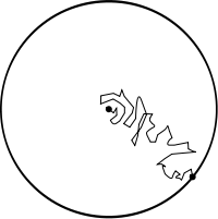
From this picture, we see that the random walk / Brownian motion in ${\mathbb{D}}$ approaches exactly one point ${u(\infty)}$ (with probability) of the Euclidean circle ${S^1=\partial\mathbb{D}}$ (working as a circle at infinity for ${\mathbb{D}}$ equipped with the hyperbolic metric, of course). In particular, we are tempted to say that ${S^1}$ is the natural boundary obtained from random walks on (the symmetric space ${\mathbb{H}}$ of) ${SL(2,\mathbb{R})}$ .

The discussion of the previous paragraphs can be summarized as follows. We started with ${G=SL(2,\mathbb{R})}$ and we considered certain (“nice”) group invariant random walks ${u_n}$ . Then, we attached a boundary space ${B=S^1}$ to form a topological space ${G\cup B}$ in such a way that ${u_n}$ converges to a point in ${B}$ with probability ${1}$ . Note that this permits to define a continuous ${G}$ -action on ${B}$ by setting ${g(b)=\lim\limits_{n\rightarrow\infty}g(u_n)}$ if ${b=\lim\limits_{n\rightarrow\infty}u_n}$ . In the literature, one then says that ${B}$ is a ${G}$ –space.

Actually, the boundary space ${B}$ comes with a natural probability measure ${\nu}$ corresponding to the distribution of ${\lim\limits_{n\rightarrow\infty} u_n}$ . For our purposes, it is important to consider ${(B,\nu)}$ (and not only the topological ${G}$ -space ${B}$ alone) and, for this reason, what we will call Poisson boundary will be ${(B,\nu)}$ .

After this informal description of the features of the Poisson boundary, let us try to formalize this notion.

3. Formal description of the Poisson boundary

From now on, let us fix ${G}$ be a locally compact group with a countable basis of open sets and ${\mu}$ a probability measure on ${G}$ . The basic examples to keep in mind are:

${G}$ a group of matrices (e.g., ${SL(n,\mathbb{R})}$ ) and ${\mu}$ a probability measure on ${G}$ that is absolutely continuous with respect to Haar measure;
${G}$ is a discrete group (e.g., ${SL(n,\mathbb{Z})}$ ) and ${\mu}$ is a countable sequence of non-negative weights ${\mu(g)}$ , ${g\in G}$ , such that ${\sum_{g\in G}\mu(g)=1}$ .

We want to attach a ${G}$ -space ${B}$ to ${G}$ in such a way that ${G\cup B}$ is still a ${G}$ -space and a group invariant random walk with law ${\mu}$ in ${G}$ converges to a point in ${B}$ with probability ${1}$ .

As it is usual, one can get an idea of what kind of space ${B}$ should be by assuming that ${B}$ was already constructed and then by trying to extract several properties that ${B}$ must satisfy hoping that this set of properties “determine” ${B}$ .

Let us try this approach now.

3.1. Definition of a boundary of ${(G,\mu)}$

We start by describing what is the class of random walks that we want to look at in order to extract limits. Consider the product probability space

$\displaystyle (\Omega,\mathcal{B},P)=(G,\mathcal{B}(G),\mu)\times\dots\times(G,\mathcal{B}(G),\mu)\times\dots=(G,\mathcal{B}(G),\mu)^{\mathbb{N}}$

We represent the points of ${\Omega}$ as ${(x_1,x_2,\dots,x_n,\dots)\in\Omega}$ and we observe that, by definition, the coordinate functions ${x_i:\Omega\rightarrow G}$ are independent ${G}$ -valued random variable with distribution ${\mu}$ . We refer to ${\{x_i\}_{i\in\mathbb{N}}}$ as a stationary sequence of independent random variables with distribution ${\mu}$ .

We now form the product random variables ${u_n=x_1 x_2\dots x_n}$ . The sequence ${\{u_n\}}$ is a Markov process as the probability of a sequence of steps ${u_1\rightarrow u_2\rightarrow \dots\rightarrow u_n\rightarrow u_{n+1}}$ is the product of the probabilities of the individual transitions ${u_i\rightarrow u_{i+1}}$ . Moreover, the transitions ${u_m\rightarrow u_{m+1}}$ in the sequence ${\{u_n\}}$ are given by (right) group multiplication: ${u_{m+1}=u_m x_{m+1}}$ . For this reason, we call the sequence of product random variables ${\{u_n\}}$ a random walk in ${G}$ with law ${\mu}$ . By the way, note that this setting is entirely determined from the data of ${G}$ and ${\mu}$ .

The scenario provided by ${\{u_n\}}$ is almost the one that we want to consider. Indeed, we said “almost” only because the group invariance is missing in the picture, that is, we want to consider all random walks ${gu_n}$ with ${g\in G}$ in order to get a setting that is invariant under (left) group multiplication.

In summary, given ${G}$ and ${\mu}$ , our group invariant random walk consists of the random variables ${gu_n}$ with ${g\in G}$ and ${\{u_n\}}$ as above.

Next, let us suppose that we have a ${G}$ -space ${B}$ such that ${G\cup B}$ is a ${G}$ -space and the group invariant random walk ${gu_n}$ converges to a point in ${B}$ with probability ${1}$ . For later use, let us observe that if the random variables ${u_n=x_1\dots x_n}$ converge to a ${B}$ -valued random variable ${z_1}$ , then ${gu_n}$ converges to ${gz_1}$ . In particular, for each ${k\in\mathbb{N}}$ , the sequence ${x_k x_{k+1}\dots x_n}$ converges to a ${B}$ -valued random variable ${z_k}$ with the following properties:

(i) ${z_k = x_k z_{k+1}}$ (by the definition of ${z_k}$ and the fact that ${G\cup B}$ is a ${G}$ -space);
(ii) ${z_k}$ is a function of ${x_k, x_{k+1}, \dots}$ (by definition);
(iii) all ${z_k}$ ‘s have the same distribution (by the group invariance of ${gu_n}$ );
(iv) ${x_k}$ is independent of ${z_{k+1},\dots}$ (by item (ii) and the independence of ${x_i}$ ‘s);

In the literature, a sequence of random variables ${\{z_n\}}$ on a ${G}$ -space ${B}$ satisfying items (i), (ii), (iii) and (iv) above is called a ${\mu}$ –process.

In this language, we just saw that any candidate ${B}$ for a (Poisson) boundary of ${G}$ must be a ${G}$ -space equipped with a ${\mu}$ -process.

Let us now investigate more closely the properties of the ${\mu}$ -process ${\{z_n\}}$ associated to a “(Poisson) boundary candidate” ${B}$ .

Denote by ${\nu}$ the distribution of an arbitrary ${z_n}$ (by item (iii) they have all the same distribution). In particular, the relation ${z_k=x_k z_{k+1}}$ (from item (i)) implies that the random variable ${x_k z_{k+1}}$ has distribution ${\nu}$ .

On the other hand, given a ${G}$ -space ${T}$ and two random variables ${x:\Omega\rightarrow G}$ and ${y:\Omega\rightarrow T}$ with distributions ${\mu}$ and ${\nu}$ , it is not hard to check that the distribution of the ${T}$ -valued random variable ${xy:\Omega\rightarrow T}$ is the convolution ${\mu\ast\nu}$ measure defined by:

$\displaystyle \int_{T} f(t)d\mu\ast\nu(t)=\int_G\int_T f(gt)d\nu(t)d\mu(g).$

Hence, since ${x_k}$ has distribution ${\mu}$ , we deduce from the equality ${z_k=x_k z_{k+1}}$ that

$\displaystyle \mu\ast\nu=\nu,$

or, in probabilistic nomenclature, ${\nu}$ is a ${\mu}$ –stationary measure.

In principle, it seems that the ${\mu}$ -process ${\{z_n\}}$ is more important (in the study of Poisson boundaries) than the stationary measure ${\nu}$ . However, the following proposition shows that one can recover the topological structure of ${G\cup B}$ from the knowledge of ${\nu}$ thanks to the martingale convergence theorem.

Proposition 5 If ${\{z_n\}}$ is a ${\mu}$ -process with distribution ${\nu}$ , then

$\displaystyle (x_1\dots x_n)_*(\nu)\rightarrow \delta_{z_1}$

with probability ${1}$ .

Here, ${g_*(\nu):=\delta_g\ast\nu}$ denotes the push-forward of ${\nu}$ by ${g\in G}$ and the convergence of the measures is in the weak- ${\ast}$ topology.

Proof: Let ${f}$ be a test (bounded, continuous) function on the ${G}$ -space ${B}$ . By definition of weak- ${\ast}$ convergence, our task consists into showing that

$\displaystyle \int_B f(\xi) d(x_1\dots x_n)_*(\nu)(\xi):=\int_B f(x_1\dots x_n \xi) d\nu(\xi) \rightarrow f(z_1)$

as ${n\rightarrow \infty}$ with probability ${1}$ .

We claim that this is a consequence of the martingale convergence theorem that the integrable random variable ${f(z_1)=f(z_1(x_1, x_2, \dots))}$ satisfies

$\displaystyle \mathbb{E}(f(z_1)|x_1, x_2,\dots, x_n)\rightarrow f(z_1)$

as ${n\rightarrow\infty}$ with probability ${1}$ where ${\mathbb{E}}$ denotes the conditional expectation.

Indeed, let us recall that ${z_1=x_1\dots x_n z_{n+1}}$ (cf. item (i) above) where ${x_1,\dots, x_n}$ and ${z_{n+1}}$ are independent (cf. item (iv) above), and ${z_{n+1}}$ has distribution ${\nu}$ (cf. item (iii) above). By plugging this into the definition of conditional expectation, we obtain the equality

$\displaystyle \int_B f(x_1\dots x_n \xi) d\nu(\xi) = \mathbb{E}(f(x_1\dots x_n z_{n+1})|x_1,\dots, x_n) = \mathbb{E}(f(z_1)|x_1,\dots, x_n),$

so that the desired convergence follows from the martingale convergence theorem. $\Box$

In other words, this proposition allows to recover the limit relation ${x_1\dots x_n\rightarrow z_1}$ , i.e., the topology of ${G\cup B}$ from the ${\mu}$ -stationary measure ${\nu}$ by identifying the points ${z_1}$ of ${B}$ with Dirac masses ${\delta_{z_1}}$ and by analyzing the convergence of the sequence of push-forwards ${(x_1\dots x_n)_*(\nu)}$ to Dirac masses ${\delta_{z_1}}$ . This observation motivates the following definition. Given ${B}$ a ${G}$ -space equipped with a probability measure ${\nu}$ , the measure topology of ${G\cup B}$ with respect to ${\nu}$ is the weakest topology such that the natural inclusions ${G\rightarrow G\cup B}$ and ${B\rightarrow G\cup B}$ are homeomorphisms into their images, and the map ${m:G\cup B\rightarrow \mathcal{M}(B)}$ from ${G\cup B}$ to the space ${\mathcal{M}(B)}$ of probability measures on ${B}$ given by ${m(g)=g_*(\nu)}$ for ${g\in G}$ and ${m(\xi)=\delta_{\xi}}$ is continuous.

At this point, our discussion so far can be summarized as follows. The investigation of the properties of a potential candidate to (Poisson) boundary ${B}$ led us to the notion of ${\mu}$ -process ${\{z_k\}}$ , and, in some sense, ${\mu}$ -processes are the right object to look at because Proposition 5 says that a ${\mu}$ -process on ${B}$ allows to think of ${B}$ as boundary after endowing ${G\cup B}$ with the measure topology with respect to the distribution of the ${\mu}$ -process.

For this reason, we introduce the following definition:

Definition 6 A ${G}$ -space ${B}$ equipped with a ${\mu}$ -stationary measure ${\nu}$ is a boundary of ${(G,\mu)}$ if ${\nu}$ is the distribution of a ${\mu}$ -process on ${B}$ .

Given this scenario, it is natural to ask whether a given ${G}$ -space ${B}$ admits some ${\mu}$ -process. The next proposition says that we already know the answer to this question.

Proposition 7 Let ${\nu}$ be a ${\mu}$ -stationary measure on a ${G}$ -space ${B}$ (i.e., ${\mu\ast\nu=\nu}$ ). Then, there exists a ${\mu}$ -process on ${B}$ with distribution ${\nu}$ if and only if the sequence ${(x_1 x_2\dots x_n)_*(\nu)}$ converges to Dirac masses on ${B}$ .

Proof: The implication ${\implies}$ was already shown in Proposition 5. For the converse implication, let us set ${\delta_{z_k}:=\lim\limits_{n\rightarrow\infty}(x_k\dots x_{k+n})_*(\nu)}$ . The sequence of random variables ${\{z_k\}}$ satisfies items (i) (by continuity of the push-forward operation under continuous transformations), (ii) (by definition) and (iv) (by item (ii) and independence of ${x_k}$ ‘s). Also, item (iii) follows from the fact that the sequences ${x_1, x_2, \dots}$ and ${x_{k}, x_{k+1}, \dots}$ have the same probabilistic behavior.

In particular, it remains only to check that the distribution of ${z_k}$ is ${\nu}$ . For this sake, we take a test function ${f}$ and we notice that

$\displaystyle \mathbb{E}(f(z_1)) = \lim\limits_{n\rightarrow\infty} \mathbb{E}\left(\int f(x_1x_2\dots x_n\xi)d\nu(\xi)\right) = \lim\limits_{n\rightarrow\infty}\int f(\xi) d(\mu^n\ast\nu)(\xi)$

Here, ${\mu^n=\underbrace{\mu\ast\dots\ast\mu}_{n}}$ and, in the last equality, we used the fact that the distribution of ${xy}$ is ${\mu\ast\nu}$ if ${x}$ has distribution ${\mu}$ and ${y}$ has distribution ${\nu}$ . Now, since ${\nu}$ is ${\mu}$ -stationary, we deduce that

$\displaystyle \int f(\xi) d(\mu^n\ast\nu)(\xi) = \int f(\xi) d\nu(\xi)$

for all ${n\in\mathbb{N}}$ . Therefore, we showed that ${\mathbb{E}(f(z_1))=\int f(\xi)d\nu(\xi)}$ , i.e., ${z_1}$ has distribution ${\nu}$ . $\Box$

3.2. Definition of the Poisson boundary of ${(G,\mu)}$

For our purposes, we want the Poisson boundary of ${(G,\mu)}$ to be a boundary that is as “large” as possible: intuitively, the large boundary sees the fine properties of ${(G,\mu)}$ , and, in particular, we can expect to distinguish between several groups (such as the lattices of ${SL(2,\mathbb{R})}$ and ${SL(r,\mathbb{R})}$ , ${r\geq 3}$ ) by looking at their largest boundaries.

3.2.1. Equivariant images

In order to “compare” boundaries, we consider equivariant maps between them: given two boundaries ${(B,\nu)}$ and ${(B',\nu')}$ of ${(G,\mu)}$ , we say that ${(B',\nu')}$ is an equivariant image of ${(B,\nu)}$ if there is an equivariant map ${\rho:B\rightarrow B'}$ (i.e., a map such that ${\rho(g\xi)=g\rho(\xi)}$ for all ${\xi\in B}$ and ${g\in G}$ ) such that ${\rho_*(\nu)=\nu'}$ .

Remark 2 This definition makes sense as the notion of equivariant image preserves boundaries: in fact, if ${\{z_n\}}$ is a ${\mu}$ -process on ${B}$ , then ${z_n'=\rho(z_n)}$ is a ${\mu}$ -process on ${B'}$ .

In the light of this definition, it is tempting to say that the Poisson boundary of ${(G,\mu)}$ is the “largest” boundary ${(B,\nu)}$ in the sense that all other boundaries ${(B',\nu')}$ can be obtained as equivariant images of ${(B,\nu)}$ .

As it turns out, this is an almost complete description of the Poisson boundary. Indeed, before giving the complete definition, we will need to discuss ${\mu}$ –harmonic functions on ${G}$ because, as we will see, they are important objects in the construction of Poisson boundaries.

Here, the basic idea is that we can “recover” a space ${B}$ from the knowledge of the functions on it. In the particular case that ${B}$ is a ${G}$ -space such that ${G\cup B}$ is a ${G}$ -space and ${gx_1\dots x_n}$ converges with probability ${1}$ (i.e., ${B}$ is a candidate to be a boundary), a continuous function ${f(g)}$ extending to a continuous function on ${G\cup B}$ has the property that ${f(gx_1\dots x_n)}$ converges with probability ${1}$ . Thus, we can “recover” information on ${B}$ from the class ${\mathcal{A}}$ of functions ${f}$ on ${G}$ with the property that ${f(gx_1\dots x_n)}$ converges with probability ${1}$ (because these functions “induce” functions on ${B}$ ). Of course, the main point of the class ${\mathcal{A}}$ is that it is canonically attached to ${(G,\mu)}$ and hence it is natural to use ${\mathcal{A}}$ to produce reference (Poisson) boundaries. In this setting, the ${\mu}$ -harmonic functions that we mentioned above are an interesting subclass of the class ${\mathcal{A}}$ .

3.2.2. ${\mu}$ -harmonic functions on ${G}$

A ${\mu}$ -harmonic function is a function satisfying the following analog of the mean value property for classical harmonic functions:

Definition 8 A bounded measurable function ${h}$ on ${G}$ is ${\mu}$ -harmonic if

$\displaystyle h(g)=\int_{G} h(gg')d\mu(g')$

for all ${g\in G}$ . We denote by ${\mathcal{H}}$ the class of ${\mu}$ -harmonic functions.

Remark 3 Since the stationary sequence of independent random variables ${\{x_n\}}$ has distribution ${\mu}$ , we have that any ${h\in\mathcal{H}}$ satisfies

$\displaystyle \mathbb{E}(h(gx_n)) = h(g)$

for each ${n\in\mathbb{N}}$ .

The following proposition says that the class ${\mathcal{H}}$ of ${\mu}$ -harmonic functions is a subclass of the class ${\mathcal{A}}$ of bounded measurable functions ${f}$ such that ${f(gx_1\dots x_n)}$ converges with probability ${1}$ .

Proposition 9 For each ${g\in G}$ , let ${w_0=h(g)}$ and ${w_n=h(gx_1\dots x_n)}$ where ${h\in\mathcal{H}}$ (i.e., ${h}$ is ${\mu}$ -harmonic). Then, ${w_n}$ converges with probability ${1}$ and ${w_{\infty}:=\lim\limits_{n\rightarrow\infty} w_n}$ satisfies

$\displaystyle \mathbb{E}(w_\infty)=h(g)$

Proof: Similarly to Proposition 5, this proposition is a consequence of the martingale convergence theorem. More concretely, the scheme of the proof is the following. We will show below that ${w_n}$ converges in ${L^2(\Omega,P)}$ (where ${(\Omega,P)=(G,\mu)^{\mathbb{N}}}$ ) to ${w_{\infty}}$ , and ${\mathbb{E}(w_{\infty}| x_1,\dots, x_k)=w_k}$ for ${k\in\mathbb{N}}$ . In particular, since the martingale convergence theorem ensures that ${\mathbb{E}(w_{\infty}|x_1,\dots,x_k)}$ converges to ${w_{\infty}}$ with probability ${1}$ , the first assertion of the proposition will then follow.

Let us now show that ${w_n\rightarrow w_{\infty}}$ in ${L^2}$ . Set ${\Delta_0=w_0}$ and ${\Delta_n=w_n-w_{n-1}}$ . We claim that the ${\Delta_n}$ ‘s are mutually ${L^2}$ -orthogonal. Indeed, by Remark 3,

$\displaystyle \mathbb{E}(h(gx_1\dots x_{n})| x_1,\dots,x_{n-1})=h(gx_1\dots x_{n-1})$

so that ${\mathbb{E}(\Delta_n|x_1,\dots,x_{n-1})=0}$ for each ${n\in\mathbb{N}}$ .

Now, let us use this information to compute the ${L^2}$ -inner product ${\mathbb{E}(\Delta_n\overline{\Delta}_{n-i})}$ between ${\Delta_n}$ and ${\Delta_{n-i}}$ for ${i>0}$ . By letting the variables ${x_1, \dots, x_{n-1}}$ fixed while allowing ${x_n}$ to vary, we see that ${\overline{\Delta}_{n-i}}$ is fixed and only ${\Delta_n}$ varies. In particular, by performing first the integration with respect to ${x_n}$ in the integral defining ${\mathbb{E}(\Delta_n\overline{\Delta}_{n-i})}$ , we deduce that ${\mathbb{E}(\Delta_n\overline{\Delta}_{n-i})}$ is a multiple of ${\mathbb{E}(\Delta_n|x_1,\dots,x_{n-1})=0}$ (by the previous paragraph), i.e., the random variables ${\Delta_n}$ are mutually ${L^2}$ -orthogonal.

From this ${L^2}$ -orthogonality, we get

$\displaystyle \|\Delta_0\|_{L^2}+\dots+\|\Delta_n\|_{L^2}=\|\sum\limits_{j=0}^n\Delta_j\|_{L^2}=\|w_n\|_{L^2}\leq \|h\|_{L^{\infty}}$

In particular, ${w_n=\sum\limits_{j=0}^n\Delta_j}$ has a limit in ${L^2}$ that we denote by ${w_{\infty}}$ .

As we already mentioned, the first assertion of the proposition will follow (from the martingale convergence theorem) once we show that ${\mathbb{E}(w_{\infty}| x_1,\dots, x_k)=w_k}$ for ${k\in\mathbb{N}}$ . In this direction, we observe that ${\mathbb{E}(\Delta_j|x_1,\dots,x_k)=0}$ for all ${j>k}$ (cf. Remark 3). By putting this together with the ${L^2}$ -orthogonality of ${\Delta_n}$ ‘s (and the fact that ${w_n=\sum\limits_{j=0}^n\Delta_j}$ by definition), we obtain that

$\displaystyle \mathbb{E}(w_n|x_1,\dots,x_k)=w_k$

for all ${n\geq k}$ . Therefore, by the ${L^2}$ -convergence of ${w_n}$ to ${w_{\infty}}$ , we conclude that

$\displaystyle \mathbb{E}(w_{\infty}|x_1,\dots,x_{k})=w_k$

so that the proof of the proposition is complete. $\Box$

For later use, we will note that a ${\mu}$ -harmonic function is determined by its boundary values (similarly to Poisson’s formula for classical harmonic functions):

Proposition 10 Let ${\nu}$ be a ${\mu}$ -stationary measure on a ${G}$ -space ${B}$ . Then, given ${\phi}$ a bounded measurable function on ${B}$ , the function

$\displaystyle h_{\phi}(g)=h(g):=\int_{B} \phi(g\xi)d\nu(\xi)$

is ${\mu}$ -harmonic.

Proof: By definition, given ${g\in G}$ ,

$\displaystyle \int_G h(gg') d\mu(g')=\int_G \int_B \phi(gg'\eta)d\nu(\eta)d\mu(g')$

By performing the change of variables ${\xi=g\eta}$ and using the definition of the convolution measure ${\mu\ast\nu}$ , we see that

$\displaystyle \int_G h(gg') d\mu(g')=\int_G \int_B \phi(gg'\eta)d\nu(\eta)d\mu(g') = \int_B \phi(g\xi) d(\mu\ast\nu)(\xi)$

Since ${\nu}$ is ${\mu}$ -stationary, i.e., ${\mu\ast\nu=\nu}$ , we deduce that

$\displaystyle \int_G h(gg') d\mu(g') = \int_B \phi(g\xi) d(\mu\ast\nu)(\xi) = \int_B \phi(g\xi) d\nu(\xi) = h(g),$

that is, ${h}$ is ${\mu}$ -harmonic. $\Box$

Corollary 11 Let ${B}$ be a compact ${G}$ -space equipped with a ${\mu}$ -stationary probability measure ${\mu}$ . Then, the sequence of probability measures ${(x_1\dots x_n)_*(\nu)}$ converges in ${\mathcal{M}(B)}$ with probability ${1}$ .

Proof: We want to show that the sequence ${(x_1\dots x_n)_*(\nu)}$ converges in ${\mathcal{M}(B)}$ with probability ${1}$ . For this sake, it is sufficient to check that, with probability ${1}$ , the integrals

$\displaystyle \int_B \phi(\xi) d(x_1\dots x_n)_*(\nu)(\xi)$

converge for all continuous functions ${\phi}$ on ${B}$ .

Given a continuous function ${\phi}$ on ${B}$ , by Proposition 10 we have that

$\displaystyle \int_B \phi(\xi) d(x_1\dots x_n)_*(\nu)(\xi):=\int_B \phi(x_1\dots x_n\xi)d\nu(\xi) = h_{\phi}(x_1\dots x_n)$

where the function ${h_{\phi}}$ is ${\mu}$ -harmonic.

It follows from Proposition 9 that ${\int_B \phi(\xi) d(x_1\dots x_n)_*(\nu)(\xi)=h_{\phi}(x_1\dots x_n)}$ converges with probability ${1}$ and this almost complete the proof of the corollary.

Indeed, we showed that, for each continuous function ${\phi}$ on ${B}$ , there exists a set ${\Omega_{\phi}}$ with full probability such that the integrals ${\int_B \phi(\xi) d(x_1\dots x_n)_*(\nu)(\xi)}$ converge whenever ${(x_1, x_2,\dots)\in\Omega_{\phi}}$ . However, the quantifiers in the last phrase do not correspond to the statement in the corollary as the latter asks for a set ${\Omega_{\infty}}$ of full probability working for all continuous functions ${\phi}$ on ${B}$ at once! Fortunately, this little technical problem is not hard to overcome: since ${B}$ is a compact (Hausdorff) space, the space of continuous functions on ${B}$ has a countable dense subset ${\{\phi_i\}_{i\in\mathbb{N}}}$ ; in particular, by setting

$\displaystyle \Omega_{\infty}:=\bigcap\limits_{i\in\mathbb{N}}\Omega_{\phi_i}$

we get a full probability set such that, for all continuous ${\phi}$ , the integrals

$\displaystyle \int_B \phi(\xi) d(x_1\dots x_n)_*(\nu)(\xi)$

converge whenever ${(x_1, x_2,\dots)\in\Omega_{\infty}}$ . $\Box$

At this stage, we are ready to give the definition of the Poisson boundary of ${(G,\mu)}$ .

3.2.3. Definition of the Poisson boundary

We say that a boundary ${(B,\nu)}$ of ${(G,\mu)}$ is the Poisson boundary if:

(a) ${(B,\nu)}$ is maximal: every boundary ${(B',\nu')}$ of ${(G,\mu)}$ is an equivariant image of ${(B,\nu)}$ .
(b) Poisson’s formula induces an isomorphism: if ${h(g)}$ is a ${\mu}$ -harmonic function on ${G}$ , there exists a bounded measurable function ${\hat{h}(\xi)}$ on ${B}$ such that
$\displaystyle h(g)=\int_B \hat{h}(g\xi) d\nu(\xi);$

moreover, ${\hat{h}}$ is unique modulo ${\nu}$ -nullfunctions, i.e., measurable functions vanishing ${\nu}$ -almost everywhere.

Completing our discussion so far, we will show in next section that the Poisson boundary always exists.

4. Construction of Poisson boundary

The main result of this section is:

Theorem 12 (Furstenberg (1963)) Let ${G}$ be a locally compact group with a countable basis of open sets and let ${\mu}$ be a probability measure on ${G}$ . Then, ${(G,\mu)}$ admits a Poisson boundary ${(B,\nu)}$ .

Proof: The basic strategy to construct ${(B,\nu)}$ using the class ${\mathcal{H}}$ of ${\mu}$ -harmonic functions.

However, we will not work exclusively with ${\mathcal{H}}$ and, in fact, we will use also the slightly larger class ${\mathcal{A}(\supset\mathcal{H}) }$ of bounded measurable functions ${f}$ on ${G}$ such that ${\lim\limits_{n\rightarrow\infty} f(g x_1\dots x_n)}$ exists with probability ${1}$ . Indeed, from the technical point of view, the main advantage of ${\mathcal{A}}$ over ${\mathcal{H}}$ is the fact that ${\mathcal{A}}$ is a Banach algebra (with respect to the ${L^{\infty}}$ -norm) while ${\mathcal{H}}$ is not.

Nevertheless, ${\mathcal{H}}$ is not “very different” from ${\mathcal{A}}$ . More precisely, let ${\mathcal{I}}$ be the ideal of ${\mathcal{A}}$ consisting of the functions ${f\in\mathcal{A}}$ such that ${f(gx_1\dots x_n)}$ converges to zero with probability ${1}$ .

Lemma 13 ${\mathcal{A}=\mathcal{H}\oplus\mathcal{I}}$ . In particular, ${\mathcal{H}\simeq\mathcal{A}/\mathcal{I}}$ .

For the proof of this lemma (and also for later use), we will need the auxiliary class ${\mathcal{L}}$ of limit functions ${z_g(x_1,\dots, x_n,\dots)=\lim\limits_{n\rightarrow\infty} f(gx_1\dots x_n)}$ corresponding to the “boundary values” of functions ${f\in\mathcal{A}}$ . Note that ${\mathcal{L}}$ is also a Banach algebra and ${\mathcal{L}\simeq\mathcal{A}/\mathcal{I}}$ .

Proof: Given ${f\in\mathcal{A}}$ , we can produce a ${\mu}$ -harmonic function ${h}$ by letting ${z_g=\lim\limits_{n\rightarrow\infty} f(gx_1\dots x_n)}$ and ${h(g):=\mathbb{E}(z_g)}$ . Indeed, the ${\mu}$ -harmonicity of ${h}$ can be checked as follows. Let ${x_0}$ be a random variable independent of the random variables ${x_n}$ ‘s on ${(\Omega, P)=(G,\mu)^{\mathbb{N}}}$ with distribution ${\mu}$ . Consider the expression ${\mathbb{E}(h(gx_0))}$ . Since the sequences ${x_0, x_1, \dots, x_n, \dots}$ and ${x_1,\dots, x_n, \dots}$ are probabilistically equivalent, we have that

$\displaystyle \mathbb{E}(h(gx_0)) = \mathbb{E}(\lim\limits_{n\rightarrow\infty} f(g x_0 x_1\dots x_n))=h(g)$

Let us now show that ${f-h\in\mathcal{I}}$ (so that ${f=h+(f-h)}$ with ${h\in\mathcal{H}}$ and ${f-h\in\mathcal{I}}$ ). By repeating the “shift of variables” argument of the previous paragraph, we see that

$\displaystyle h(gx_1\dots x_n) = \mathbb{E}(\lim\limits_{n\rightarrow\infty} f(gx_1\dots x_n x_{n+1}\dots)|x_1,\dots, x_n) = \mathbb{E}(z_g|x_1,\dots,x_n).$

On the other hand, the martingale convergence theorem says that ${z_g=\lim\limits_{n\rightarrow\infty}\mathbb{E}(z_g|x_1,\dots,x_n)}$ (with probability ${1}$ ), so that we deduce that

$\displaystyle \lim\limits_{n\rightarrow\infty} h(gx_1\dots x_n) = z_g:=\lim\limits_{n\rightarrow\infty}f(gx_1\dots x_n)$

(with probability ${1}$ ). In particular, this means (by definition) that ${f-h\in\mathcal{I}}$ .

Completing the proof of the lemma, it remains to verify that ${\mathcal{H}\cap\mathcal{I}=\{0\}}$ . This fact follows immediately from Proposition 9 saying that a ${\mu}$ -harmonic function can be recovered from its boundary values. $\Box$

From this lemma, we have that ${\mathcal{H}\simeq\mathcal{A}/\mathcal{I}\simeq\mathcal{L}}$ . Now, note that ${\mathcal{A}/\mathcal{I}}$ is a commutative ${C^*}$ -algebra, so that it has a representation as the space ${C^0(\widetilde{B})}$ of continuous function on a compact (Hausdorff) space ${\widetilde{B}}$ (called the spectrum of ${\mathcal{A}/\mathcal{I}}$ ) by Gelfand’s representation theorem.

From this, we deduce two consequences: firstly, we have a correspondence between ${\mu}$ -harmonic functions ${h(g)}$ on ${G}$ and continuous functions ${\widetilde{h}(\eta)}$ on ${\widetilde{B}}$ ; secondly, the “evaluation at identity” functional ${ev_e}$ associating to each ${\mu}$ -harmonic function ${h}$ is value at ${e\in G}$ , i.e., ${ev_e(h)=h(e)}$ is a linear functional that is non-negative (that is, it takes non-negative values on non-negative elements of ${\mathcal{A}/\mathcal{I}}$ ) and it takes the constant function ${1}$ to the real value ${1}$ , so that, by Riesz representation theorem, there exists an unique probability measure ${\widetilde{\nu}}$ on ${\widetilde{B}}$ such that

$\displaystyle ev_e(h)=\int_{\widetilde{B}} \widetilde{h}(\eta) d\widetilde{\nu}(\eta).$

Note that ${\widetilde{B}}$ is a ${G}$ -space as the natural action of ${G}$ on ${\mathcal{A}}$ via ${f(.)\in\mathcal{A}\mapsto f(g.)}$ for each ${g\in G}$ sends ${\mathcal{I}}$ into itself. Also, if a ${\mu}$ -harmonic function ${h(g)}$ corresponds to ${\widetilde{h}(\eta)}$ , then ${h(g_0 g)}$ corresponds to ${\widetilde{h}(g_0\eta)}$ . In particular, the formula above for ${ev_e}$ gives the following Poisson formula:

$\displaystyle h(g)=\int_B \widetilde{h}(g\eta) d\widetilde{\nu}(\eta) \ \ \ \ \ (1)$

A pleasant point about the construction of ${(\widetilde{B},\widetilde{\nu})}$ is that it is canonical (i.e., it leads to an unique object) and, in particular, it is tempting to use ${(\widetilde{B}, \widetilde{\nu})}$ as the Poisson boundary.

However, this does not work because ${\widetilde{B}}$ is too “large”, i.e., it might not have a countable basis of open sets. So, the notions of convergence of sequences of points or measures is not “natural” for a technical reason that we already encountered in the end of the proof of Corollary 11. Namely, when trying to prove that a sequence of measures ${\theta_n}$ (depending on ${(x_1,x_2,\dots)\in \Omega=G^{\mathbb{N}}}$ ) on ${\widetilde{B}}$ converges with probability ${1}$ , we will show that for each continuous function ${\psi}$ there exists a full measure set ${\Omega_{\phi}}$ such that the integrals ${\int \psi(\eta) d\theta_n(\eta)}$ converges for any element of ${\Omega_{\phi}}$ , but if ${\widetilde{B}}$ has no countable basis, we can’t select a countable dense set ${\{\phi_i\}}$ of continuous functions and, hence, we can’t conclude that the integrals ${\int \psi(\eta) d\theta_n(\eta)}$ converge with probability ${1}$ via the usual argument of taking ${\Omega_{\infty}=\bigcap\limits_{i\in\mathbb{N}}\Omega_{\phi_i}}$ .

To overcome this difficulty, we observe that ${G}$ is separable, so that the spaces ${L^p(\widetilde{B},\widetilde{\nu})}$ are separable for ${1\leq p<\infty}$ . In particular, one can find a subalgebra ${\mathcal{C}}$ of ${L^{\infty}(\widetilde{B}, \widetilde{\nu})}$ possessing a countable dense set which is also dense in ${L^p(\widetilde{B},\widetilde{\nu})}$ for all ${1\leq p<\infty}$ . Furthermore, since ${G}$ has a countable dense subset ${\{g_i\}_{i\in\mathbb{N}}}$ , we can choose the subalgebra ${\mathcal{C}}$ to be ${G}$ -invariant (by “forcing” invariance with respect to every ${g_i}$ ). Using ${\mathcal{C}}$ one can define a quotient space ${B}$ of ${\widetilde{B}}$ such that ${\mathcal{C}}$ is isomorphic to the space of continuous functions ${C^0(B)}$ . Note that ${B}$ comes equipped with a probability measure ${\nu}$ (obtained by push-forward of ${\widetilde{\nu}}$ with respect to the projection ${\widetilde{B}\rightarrow B}$ ). Moreover, since ${L^p(B,\nu)}$ is the completion of ${C^0(B)}$ with respect to the ${L^p}$ -norm and ${\mathcal{C}}$ is dense in ${L^p(\widetilde{B},\widetilde{\nu})}$ , we see that the spaces ${L^p(B,\nu)}$ and ${L^p(\widetilde{B},\widetilde{\nu})}$ are the same. In other words, the passage from ${\widetilde{B}}$ to ${B}$ makes that the class of continuous functions gets smaller, but the class of bounded measurable functions stays the same.

We claim that, by replacing ${(\widetilde{B},\widetilde{\nu})}$ by ${(B,\nu)}$ , the technical difficulty mentioned above disappears and we get the Poisson boundary of ${(G,\mu)}$ .

Let us start the proof of this claim by observing that the Poisson formula, i.e., item (b) in the definition of Poisson boundary, follows immediately from the definition of ${(B,\nu)}$ and the corresponding Poisson formula (1) for ${(\widetilde{B},\widetilde{\nu})}$ . In particular, the Poisson formula for ${(B,\nu)}$ becomes

$\displaystyle h(g)=\int_B \hat{h}(g\xi) d\nu(\xi) \ \ \ \ \ (2)$

where ${\hat{h}}$ is a bounded measurable function (corresponding to ${\widetilde{h}}$ ).

Remark 4 In fact, in item (b) of the definition of the Poisson boundary, one also requires the uniqueness of ${\hat{h}}$ modulo nullfunctions. In fact, this is not hard to show, but we will omit the details.

Next, let us check that ${\nu}$ is a ${\mu}$ -stationary measure. Note that, by definition, given a continuous function ${\hat{h}(\xi)}$ , the function

$\displaystyle h(g)=\int_B \hat{h}(g\xi) d\nu(\xi)$

is ${\mu}$ -harmonic, i.e., ${h(g)=\int_G h(gg') d\mu(g')}$ (as ${\widetilde{\nu}}$ is the measure representing the linear function ${ev_e}$ ). In particular,

$\displaystyle \int_B \hat{h}(g\xi) d\nu(\xi)= \int_G \int_B \hat{h}(gg'\eta) d\nu(\eta)d\mu(g) = \int_B \hat{h}(g\xi) d(\mu\ast\nu)(\xi),$

that is, ${\mu\ast\nu}$ and ${\nu}$ define the same linear functional from ${C^0(B)}$ to ${\mathcal{H}}$ . Therefore, ${\mu\ast\nu=\nu}$ , i.e., ${\nu}$ is ${\mu}$ -stationary.

Now, let us show that ${(B,\nu)}$ is a boundary of ${(G,\mu)}$ . By Proposition 7, our task consists in proving that ${(x_1\dots x_n)_*(\nu)}$ converges to a Dirac mass with probability ${1}$ . In this direction, note that, by Corollary 11 (applied to ${\widetilde{B}}$ and then “transferred” to ${B}$ ), we know that ${(x_1\dots x_n)_*(\nu)}$ converges to some probability measure ${\theta}$ (with probability ${1}$ ). So, it remains to show that ${\theta}$ is a Dirac mass with probability ${1}$ . For this sake, let us fix ${\phi\in C^0(B)}$ a test function and let us denote by ${h=h_{\phi}}$ the corresponding ${\mu}$ -harmonic function. From the Poisson formula (2), we get that

$\displaystyle \int_B\phi(g\xi)d\theta(\xi) = \lim\limits_{n\rightarrow\infty}\int_B\phi(gx_1\dots x_n\xi) d\nu(\xi) = \lim\limits_{n\rightarrow\infty} h(gx_1\dots x_n):=z_g\in\mathcal{L}$

On the other hand, the isomorphism between ${\mathcal{L}\simeq\mathcal{A}/\mathcal{I}}$ and the functions on ${B}$ is an algebra isomorphism. In particular,

$\displaystyle z_g^2=\int_B (\phi(g\xi))^2 d\theta(\xi)\geq \left(\int_B \phi(g\xi)d\theta(\xi)\right)^2=z_g^2,$

that is, we have equality in Cauchy-Schwarz inequality. It follows that ${\phi(\xi)}$ is ${\nu}$ -almost everywhere constant. Since this occurs for all continuous function ${\phi\in C^0(B)}$ , we deduce that ${\theta}$ is a Dirac mass.

Finally, we complete the sketch of proof of the theorem by showing that ${(B,\nu)}$ is maximal in the sense of item (a), i.e., any boundary ${(B_1,\nu_1)}$ is an equivariant image of ${(B,\nu)}$ . Keeping this goal in mind, we will construct a natural ${C^*}$ -algebra morphism from ${C^0(B_1)}$ into ${L^{\infty}(B)}$ , i.e., a morphism which is compatible with the natural ${G}$ -actions on both algebras and respecting the linear functionals induced by ${\nu_1}$ and ${\nu}$ . Let ${\phi\in C^0(B_1)}$ and consider the ${\mu}$ -harmonic function ${h(g)=\int_B \phi(g\xi) d\nu_1(\xi)}$ on ${G}$ . Denote by ${z_g\in\mathcal{L}}$ the limit function associated to ${h}$ and let ${\{w_n\}}$ the ${\mu}$ -process on ${(B_1,\nu_1)}$ . By Proposition 5, ${(x_1\dots x_n)_*(\nu_1)\rightarrow\delta_{w_1}}$ , and, thus,

$\displaystyle \phi(gw_1) = \lim\limits_{n\rightarrow\infty} \int_{B_1} \phi(gx_1\dots x_n\xi)d\nu_1(\xi) = \lim\limits_{n\rightarrow\infty} h(gx_1\dots x_n) = z_g.$

This formula makes it clear that the map ${\phi\mapsto z_g}$ is an algebra morphism from ${C^0(B_1)}$ into ${\mathcal{L}\simeq\mathcal{A}/\mathcal{I}}$ . Furthermore, this formula also shows that the natural actions of ${G}$ on these algebras are preserved, and, moreover, the linear functional induced by both ${\nu_1}$ and ${\nu}$ is given by ${z_g\mapsto \mathbb{E}(z_e)}$ .

This completes the proof of Furstenberg’s theorem on the existence of Poisson boundaries. $\Box$

Remark 5 The arguments above show that the measure-theoretical object ${L^{\infty}(B,\nu)}$ is uniquely determined, despite the fact that the topological space ${B}$ is not unique. Nevertheless, we will not dispense the topological structure ${B}$ in the definition of Poisson boundary because we want to think about it as a space attached to the group.

Remark 6 A “cousin” of the Poisson boundary is the so-called Martin boundary. Very roughly speaking, the Martin boundary is related to positive not necessarily bounded harmonic function while the Poisson boundary is related to bounded harmonic functions. In general, the Martin boundary is a realization of the Poisson boundary, but not vice-versa. For our current purpose (namely, the proof of Theorem 3), the Poisson boundary has the advantage that it does not change too much when we change the measure ${\mu}$ in a reasonable way, while the same is not true for the Martin boundary.

The summary of today’s post is the following. We saw that Furstenberg’s idea for the proof of his Theorem 3 (that a lattice of ${SL(2,\mathbb{R})}$ can’t be realized as a lattice of ${SL(r,\mathbb{R})}$ , ${r\geq 3}$ ) was to show that the boundary behavior of a discrete group is determined by the boundary behavior of its envelope. Of course, the formalization of this idea requires the construction of an adequate boundary and this is precisely what we did in this section.

Next time, we will discuss some examples of Poisson boundary. After that, we will relate the Poisson boundary of a lattice of ${SL(r,\mathbb{R})}$ to the Poisson boundary of ${SL(r,\mathbb{R})}$ and, then, we will complete the proof of Theorem 3.

Posted in expository, math.DS, Mathematics | Tags: $latex \mu$-process, Hillel Furstenberg, Poisson boundary, random walks, stationary measures

M	T	W	T	F	S	S
1	2	3	4	5	6	7
8	9	10	11	12	13	14
15	16	17	18	19	20	21
22	23	24	25	26	27	28
29	30	31

	Adam on Breuillard-Sert’s joint…
	Adam on Breuillard-Sert’s joint…
	Writing a Hilbert C*… on ERT16: Compact extensions
	matheuscmss on Yoccoz book collection at…
	Jairo B. on Yoccoz book collection at…

Disquisitiones Mathematicae