Last time, we saw that if  is a compact subset of reductive, real linear algebraic group
  such that the monoid
  generated by
  is Zariski dense in , then the Cartan projections
  and the Jordan projections
  associated to converge in the Hausdorff topology to the same limit
  , an object baptised “joint spectrum of ” by Breuillard and Sert.
Today, I’ll transcript below my notes of a talk by Romain Dujardin explaining to the participants of our groupe de travail some basic convexity and continuity properties of the joint spectrum. After that, we close the post with a brief discussion of the question of prescribing the joint spectrum.
As usual, all mistakes in what follows are my sole responsibility.
1. Preliminaries
Let us warm up by reviewing the setting of the previous posts of this series.
Let be a reductive real linear algebraic group and denote its rank by  . By definition, a maximal torus
  is isomorphic to
  .
.
The Cartan decomposition  (with
(with  a maximal compact subgroup of ) allows to write any
  as
as  for an unique
  where
where  is a choice of Weyl chamber in the Lie algebra
  of
of  . The interior of the Weyl chamber is denoted by
  .
.
Example 1 For  , we can take
  in
in  , so that
  .
.
The element is called the Cartan projection of  .
.
Example 2 For ,  , where
  are the singular values of .
Similarly, the Jordan projection  is defined in terms of the Jordan-Chevalley decomposition. For , this amounts to write the Jordan normal form
  with diagonalisable and
  nilpotent, so that
  with
with  unipotent,
  , and
, and  has eigenvalues
  where
where  are the eigenvalues of (ordered by decreasing sizes of their moduli).
The group has a family  of distinguished representations such that the components of the vectors
  , resp. , are linear combinations of
  , resp.
  . In particular, the usual formula for the spectral radius implies that
  as
as  (and, as it turns out, this fact is important in establishing the coincidence of the limits of the sequences and ).
Example 3 For , the representations  of on
of on  ,
,  , have the property that the eigenvalue of
  with the largest modulus is
  .
.
The rank of can be written as  where
where  is the dimension of the center
  of . In the literature,
  is called the semi-simple rank of . In general, we have “truly” distinguished representations which are completed by a choice of characters of
 ![{G/[G,G]}](https://s0.wp.com/latex.php?latex=%7BG%2F%5BG%2CG%5D%7D&bg=ffffff&fg=000000&s=0&c=20201002) .
.
Example 4 For ,  , and the representations from the previous example have the property that with
  is “truly” distinguished and the determinant representation
  comes from the center.
Remark 1 Recall that a weight  of a representation
  of is a generalized eigenvalue associated to a non-trivial -invariant subspace, i.e.,
  is a weight whenever

The weights are partially ordered via  if and only if
  for all
  , and any irreducible representation possesses an unique maximal weight
  (and, as it turns out,
  is one-dimensional).In this context, the distinguished representations
  form a family of representations whose maximal weights
  provide a basis of
  .
.
A matrix  is proximal when its projective action on
  possesses an attracting fixed point
  and a repulsive hyperplane
  . Also, an element is called –proximal if and only if the matrices are proximal for all
  (or, equivalently,
  ).
).
A matrix is  -proximal whenever
  is proximal,
  , and
, and  for all
  ,
,  (where is the Fubini-Study on the projective space ). Moreover, is
  –proximal if and only if the matrices are -proximal for all .
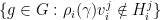
A beautiful theorem of Abels–Margulis–Soifer asserts that -proximal elements are really abundant: given a Zariski-dense monoid  of , there exists
  such that for all
  , one can find a finite subset
  with the property that for any , one can find
  with
with  -proximal.
In the previous post of this series, we saw that Abels–Margulis–Soifer was at the heart of Breuillard–Sert proof of the following result:
Theorem 1 If is compact and the monoid generated by is Zariski-dense in , then the sequences and converge in Hausdorff topology to a compact subset  called the joint spectrum of .
After this brief review of the definition of the joint spectrum, let us now study some of its basic properties.
2. Convexity of the joint spectrum
Theorem 2 is a convex subset of .
Remark 2 Later, we will see some sufficient conditions to get  .
.
Similarly to the proof of Theorem 1, some important ideas behind the proof of Theorem 2 are:
- the Jordan projection
 behaves well under powers:
  ;
;
- the Cartan projection
 is subadditive:
  ;
;
- the Cartan and Jordan projections of proximal elements are comparable: there is a constant
 such that
  for all -proximal;
- Abels–Margulis–Soifer provides a huge supply of proximal elements.
We start to formalize these ideas with the following lemma:
Lemma 3 If and  are -proximal elements, then there are
  and
and  such that
  for all
  .
.
Proof: After replacing by the matrix , our task is reduced to study the behaviours of the eigenvalues  of largest moduli of proximal matrices .
By definition of proximality, the matrices  converge to a projection
  on
on  parallel to
  as
as  . Also, an analogous statement is valid for . In particular, for any
  , one has

as .
It is not hard to show that there exists  such that
  is not nilpotent: in fact, this happens because is Zariski-dense and the nilpotency condition can be describe in polynomial terms. In particular,
  and, by continuity, there exists
  with
with
for all . This ends the proof. 
At this point, we are ready to prove Theorem 2. Since is a compact subset of , the proof of its convexity is reduced to show that  for all
  .
.
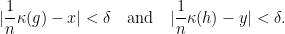
For this sake, we begin by applying Abels–Margulis–Soifer theorem in order to fix  and a finite subset
  so that for any
  we can find with
  -proximal. By definition, there exists
  such that any satisfies
  for some
  .
.
Next, we consider and we recall that  . Hence, given
  , we have that for all
  sufficiently large, there are
  with
with
Now, we select  with
with  and
and  -proximal. Recall that, by proximality, there exists a constant with

(and an analogous statement is also true for  ). Furthermore, by Lemma 3, there are , say
  , and with

for all . Observe that  .
.
By dividing by  , by taking large (so that
  ) and by letting
  (so that
  ), we see that

for and  sufficiently large.
Since is arbitrary and is closed, this proves that  . This completes the proof of Theorem 2.
3. Continuity properties of the joint spectrum
3.1. Domination and continuity
Definition 4 We say that  is
is  -dominated if there exists such that
for all sufficiently large and  . (Recall that
  are the singular values of .)
Definition 5 We say that is -dominated if  is -dominated for all .
Remark 3 If is -dominated, then it is possible to show that the joint spectrum is well-defined even when is not Zariski dense in .
The next proposition asserts that the notion of -domination generalizes the concept of matrices with simple spectrum (i.e., all of its eigenvalues have distinct moduli and multiplicity one).
Proposition 6 is -dominated if and only if  .
.
On the other hand, the notion of -domination is related to Schottky families.
Definition 7 We say that  is a -Schottky family if
- (a) any
 is -proximal;
- (b)
 for all
  .
.
Proposition 8 is -dominated  there are
  and so that
  is a -Schottky family.
Proof: Let us first establish the implication  . It is not hard to see that if is -dominated, then is -dominated. Therefore, we can assume that is a -Schottky family. At this point, we invoke the following lemma due to Breuillard–Gelander:
Lemma 9 (Breuillard–Gelander) If  is
is  -Lipschitz on an non-empty open subset
  of
of  , then
  .
.
Proof: Thanks to the  decomposition, we can assume that
  . Given
 ![{[v]\in\Omega}](https://s0.wp.com/latex.php?latex=%7B%5Bv%5D%5Cin%5COmega%7D&bg=ffffff&fg=000000&s=0&c=20201002) and sufficiently small, our assumption on implies that
and sufficiently small, our assumption on implies that ![{d([gv], [gv+\delta ge_1])<\varepsilon d([v],[v+\delta e_1])}](https://s0.wp.com/latex.php?latex=%7Bd%28%5Bgv%5D%2C+%5Bgv%2B%5Cdelta+ge_1%5D%29%3C%5Cvarepsilon+d%28%5Bv%5D%2C%5Bv%2B%5Cdelta+e_1%5D%29%7D&bg=ffffff&fg=000000&s=0&c=20201002) and
and ![{d([gv], [gv+\delta ge_2])<\varepsilon d([v],[v+\delta e_2])}](https://s0.wp.com/latex.php?latex=%7Bd%28%5Bgv%5D%2C+%5Bgv%2B%5Cdelta+ge_2%5D%29%3C%5Cvarepsilon+d%28%5Bv%5D%2C%5Bv%2B%5Cdelta+e_2%5D%29%7D&bg=ffffff&fg=000000&s=0&c=20201002) . These inequalities imply the desired fact that after some computations with the Fubini-Study metric .
. These inequalities imply the desired fact that after some computations with the Fubini-Study metric .
If is a -Schottky family, then all elements of are  -Lipschitz on a neighborhood of any fixed
  ,
,  for all . By the previous lemma, we conclude that
  for all sufficiently large and . Thus, is -dominated.
Let us now prove the implication  . For this sake, we use a result of Bochi–Gourmelon (justifying the nomenclature “domination”): is -dominated if and only if there is a dominated splitting for a natural linear cocycle over the full shift dynamics on
  , i.e.,
- Splitting condition: there are continuous maps
 and
and 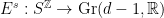 such that
  for all
  (here,
  is the Grassmannian of hyperplanes of
  );
);
- Invariance condition:
 and
and  for all
  (here,
  denotes the left shift dynamics
  );
);
- Domination condition: the weakest contraction along
 dominates the strongest expansion along
  , that is, there are
  and
and  such that
 .
.
Remark 4 For  , the equivalence between -domination and the presence of dominated splittings was established by Yoccoz.
An important metaprinciple in Dynamics (going back to the classical proofs of the stable manifold theorem) asserts that “stable spaces depend only on the future orbit”. In our present context, this is reflected by the fact that one can show that  depends only on
  and
and  depends only on
  for all .
An interesting consequence of this fact is the following statement about the “non-existence of tangencies between and ”: if is -dominated, then  for all
  . Indeed, this statement can be easily obtained by contradiction: if
  for some
  and
and  , then
  has the property that
  and
and  . Hence,
  , a contradiction with the splitting condition above.
At this stage, we are ready to show that if is -dominated, then is a -Schottky family for some and  . In fact, given , let
  be the periodic sequence obtained by infinite concatenation of the word . We affirm that, for sufficiently large, is proximal with
  and
and  , and -Lipschitz outside the -neighborhood of . This happens because the compactness of and the non-existence of tangencies between and provide an uniform transversality between and . By combining this information with the domination condition above (and the fact that
  for sufficiently large), a small linear-algebraic computation reveals that any is proximal and -Lipschitz outside the -neighborhood of for adequate choices of
  and .
and .
The proof of the previous proposition gave a clear link between -domination and the notion of dominated splittings. Since a dominated splitting is robust under small perturbations (because they are detected by variants of the so-called cone field criterion), a direct consequence of the proof of the proposition above is:
Corollary 10 The -domination property is open: if is -dominated, then any  included in a sufficiently small neighborhood of is also -dominated.
The previous proposition also links -domination to Schottky families and, as it turns out, this is a key ingredient to obtain the continuity of the joint spectrum in the presence of domination.
Theorem 11 If  is -dominated, then the map
  is continuous at .
Very roughly speaking, the proof of this result relies on the fact that if a matrix is “very Schottky” (like a huge power of a proximal matrix), then this matrix is quite close to a rank 1 operator and, in this regime, the Jordan projection behaves in an “almost additive” way.
3.2. Examples of discontinuity
3.2.1. Calculation of a joint spectrum in 
Recall that acts on Poincaré disk  by isometries of the hyperbolic metric. Consider
  , where
  and
and  are loxodromic elements of acting by translations along disjoint oriented geodesic axis
  and
and  on from
  to
to  and from
  to
to  . We assume that the endpoints of the axes and are cyclically order on
  as
as  , and we denote by
  and
and  the translation lengths of and along and .
In the sequel, we want to compute  and, for this sake, we need to understand
  where
where  is a word of length on and .
Proposition 12 If and are elements of as above,  denotes the distance between the axes of and , and
  , then is the interval
![\displaystyle J(S)=[\tau_a/2, \tau_b/2].](https://s0.wp.com/latex.php?latex=%5Cdisplaystyle+J%28S%29%3D%5B%5Ctau_a%2F2%2C+%5Ctau_b%2F2%5D.&bg=ffffff&fg=000000&s=0&c=20201002)
Proof: One can show (using hyperbolic geometry) that  is a loxodromic element whose axis stays between the axes of and while going from a point in
 ![{[x_a^-, x_b^-]}](https://s0.wp.com/latex.php?latex=%7B%5Bx_a%5E-%2C+x_b%5E-%5D%7D&bg=ffffff&fg=000000&s=0&c=20201002) to a point in
to a point in ![{[x_b^+, x_a^+]}](https://s0.wp.com/latex.php?latex=%7B%5Bx_b%5E%2B%2C+x_a%5E%2B%5D%7D&bg=ffffff&fg=000000&s=0&c=20201002) , and the translation length of satisfies
, and the translation length of satisfies

In particular,  .
.
We affirm that if is a word on and and  is a word obtained from by replacing some letter by , then
  . In fact, by performing a conjugation if necessary, we can assume that
  and
and  , so that
  and
and  .
.
Therefore, if we start in with  and we successively replace by until we reach
  , then we see from the claim in the previous paragraph that becomes denser in
 ![{[\tau_a/2, \tau_b/2]}](https://s0.wp.com/latex.php?latex=%7B%5B%5Ctau_a%2F2%2C+%5Ctau_b%2F2%5D%7D&bg=ffffff&fg=000000&s=0&c=20201002) as . This proves that
as . This proves that ![{J(S)=[\tau_a/2,\tau_b/2]}](https://s0.wp.com/latex.php?latex=%7BJ%28S%29%3D%5B%5Ctau_a%2F2%2C%5Ctau_b%2F2%5D%7D&bg=ffffff&fg=000000&s=0&c=20201002) .
.
3.2.2. Some joint spectra in 
Let  as above and fix
  . We assume that there exists such that
  where
where  is the rotation by
  .
.
The joint spectrum  of
of  in the plane with axis
  and
and  is a triangle with vertex at
  , intersecting the -axis on the interval
 ![{[\log\lambda_1(a), \log\lambda_1(b)]}](https://s0.wp.com/latex.php?latex=%7B%5B%5Clog%5Clambda_1%28a%29%2C+%5Clog%5Clambda_1%28b%29%5D%7D&bg=ffffff&fg=000000&s=0&c=20201002) , and the side opposite to the vertex contained in the line
, and the side opposite to the vertex contained in the line  . Indeed, one eventually get this description of because
  , , can be computed explicitly in terms of the joint spectrum of
  thanks to the fact that
  commutes with and . Note that
  .
.
Let us now consider  , where
  denotes the rotation by
  . We affirm that
  for all
  and, a fortiori,
  is discontinuous at
  (because
  as
as  ). In fact, given , since , the word

equals to  . Therefore,

and, by letting , we conclude that , as desired.
4. Prescribing the joint spectrum
We close this post with a brief sketch of the following result:
Theorem 13
- (1) If
 is a convex body dans , there exists a compact subset of generating a Zariski-dense monoid such that
  .
.
- (2) Moreover, if is a convex polyhedron with a finite number of vertices, then there exists a finite subset generating a Zariski-dense monoid such that .
Proof: (1) If we forget about the Zariski-denseness condition, then we could take simply  . In order to respect the Zariski-density constraint, we fix
  and we set
  where
where  is a small neighborhood of the identity. In this way, the monoid generated by is Zariski-dense and it is possible to check that whenever is sufficiently small.
(2) Given a finite set  whose convex hull is , we can take
  where
where  is a finite set with sufficiently many points so that the monoid generated by is Zariski-dense.

and the perimeter
of a smooth domain
are determined by the eigenvalues
of its Laplacian
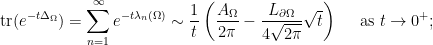
via the asymptotics of the trace of the heat operator:
, and the equality holds if and only if
.


with an arc-length parameter
, we can control the
-norms of the derivatives of the curvature
where
and, in general,
for a certain constant
and an adequate “universal” polynomial
(here,
is the
-th derivative of
for all
for all
,
into
bounds on
for all
;
, the periodic trajectories with rotation number
in the billiard table determined by
and
coincides with the set
of lengths of periodic trajectories with rotation number
, in an almost circular billiard table
and they form a caustic, so that


 (a feature which is illustrated in this numerical simulation [due to Dyatlov]
  was proved by Baladi–Demers in this article
  forces a rigidity property for periodic orbits, namely, the Lyapunov exponents of all periodic orbits coincide (note that this is a huge number of conditions because the number of periodic orbits of period
  grows exponentially with
  for certain Sinai billiards by computing the Taylor expansion of the derivative of the billiard map at a periodic orbit of period two and checking that its quadratic part is non-degenerate.
 has a probability measure of maximal entropy whenever
  (where the limit case
  corresponds to touching obstacles and the limit case
  produces “infinite horizon”).
 and
and  .
. in the direction
  travels along the line
  until it hits the boundary of the disk of radius
  for the first time
  . By definition, the time
  , i.e.,
 where
where  and
and  , the billiard trajectory starting at
 and, after a specular reflection, it takes the direction
  .
. along the following lines. If we adopt the convention in Chernov–Markarian’s book of using arc-length parametrization
  on the obstacle and describing the angle
 ![{y\in[-\pi/2,\pi/2]}](https://s0.wp.com/latex.php?latex=%7By%5Cin%5B-%5Cpi%2F2%2C%5Cpi%2F2%5D%7D&bg=ffffff&fg=000000&s=0&c=20201002) with the normal direction pointing towards the interior of the table using a sign determined by the orientation of the obstacles so that this normal vector stays at the left of the tangent vectors to the obstacles, then the billiard map becomes
with the normal direction pointing towards the interior of the table using a sign determined by the orientation of the obstacles so that this normal vector stays at the left of the tangent vectors to the obstacles, then the billiard map becomes


![{\arcsin(z)\in[-\frac{\pi}{2},\frac{\pi}{2}]}](https://s0.wp.com/latex.php?latex=%7B%5Carcsin%28z%29%5Cin%5B-%5Cfrac%7B%5Cpi%7D%7B2%7D%2C%5Cfrac%7B%5Cpi%7D%7B2%7D%5D%7D&bg=ffffff&fg=000000&s=0&c=20201002) for
for ![{z\in[-1,1]}](https://s0.wp.com/latex.php?latex=%7Bz%5Cin%5B-1%2C1%5D%7D&bg=ffffff&fg=000000&s=0&c=20201002) ) and, moreover,
) and, moreover,


 is
is
 , one has
 of the Taylor expansion of
  for
for  .
. in the limit case
  on
on  induces an action on the projective space
  . For later use, recall that
  via
via![\displaystyle \mathbb{T}^1\ni\theta\mapsto [\cos\theta:\sin\theta]=\mathbb{R}\cdot(\cos\theta,\sin\theta)\in X.](https://s0.wp.com/latex.php?latex=%5Cdisplaystyle+%5Cmathbb%7BT%7D%5E1%5Cni%5Ctheta%5Cmapsto+%5B%5Ccos%5Ctheta%3A%5Csin%5Ctheta%5D%3D%5Cmathbb%7BR%7D%5Ccdot%28%5Ccos%5Ctheta%2C%5Csin%5Ctheta%29%5Cin+X.&bg=ffffff&fg=000000&s=0&c=20201002)
 on
on  into
into  where
where  is stabilized by two elements
  , then the random walk starting at
  is not very interesting.
 .
. on
on  such that, for all
 on
on  on
on 
 is the distribution of points obtained from
 associated to
  -almost every
  whenever

 .
. is called Lyapunov exponent.
 with
with  .
.
 is the interval of radius
  centered at
  ). In particular,
 ). More concretely, he proved that:
 . In other words,
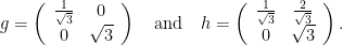
 is not Zariski dense in
  via
via  , then
  acts on
  as
as
 ,
,  , and the Fourier coefficients of the stationary measure given by the standard Hausdorff measure on middle-third Cantor set do not decay to zero.In a similar vein, if
  is a real number such that
  is a
is a  with
with
 (called the Bernoulli convolution of parameter
  where
where  with probability
  ) whose Fourier coefficients do not decay.
 , let
, let
 as a smooth version of the characteristic function of an interval
  , we see that
  is “counting random products
  ”. In this context, Guivarch and Le Page established the following renewal theorem:
 .
. of the elements of
  (whenever (i) is satisfied).
 is the
 .
.
 , consider the transfer operator
 (with
(with  small enough). Then,we have the following spectral gap property: there exists
  such that the spectral radius of
  satisfies
 .
. satisfies
 Theorem
  ;
; , the
, the 
 is reduced to the study of
 , we see that the size of the integral above depends on the “number of random products
  with norm
  in a given interval”, and the answer to this kind of “counting problem” is encoded in the asymptotic property of the renewal operator
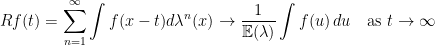
 grows polynomially with
  with
with  ,
,  , and a subset
  of
of  of cardinality
  . The corresponding set of ellipsephic integers
  is
is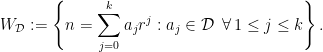

 and
and
 . Despite their sparseness, it was proved by
  and
and  such that
 ,
,  ,
,  and
and 
 . The “main term”
  comes from the case
  , so that our task consists into estimating the “error term”. For this sake, one has essentially to study
 . Observe that
 are controlled thanks to the following lemma (giving some saving over the trivial bound
  for all
  ):
): . For any
 .
. and
and  , one has
 such that for all
  there exists
  with the property that

 .
.  such that
 stands for the number of prime factors of
  in the last theorem of the previous section and, in this direction, it is possible to show that
 , then one can take
 (and
(and  ) for
) for  ,
, (and
(and  ) for
) for  , …,
, …, for
for  , and
, and as
as 
 ,
,  , then one can take
  .
. (of ellipsephic primes) in Dartyge–Mauduit theorem above. This was recently accomplished by
  and
and  , then
 digits in basis
  with two prime factors.
 and for all
  of the form
  whose largest prime factor is
  .
. such that
 (which is close to one for
  of the form:
 for all
  ), Kirsty Briggs showed that for
  prime and
  , the trivial bound
  on the number of solutions of the Vinogradov system

 can be improved into
 whenever
  . (In particular, this result is saying that in the case
  , the main contribution to the number of ellipsephic solutions of the corresponding Vinogradov system comes from the trivial solutions
  .)
.) be the power of a prime number
  and denote by
  a
a  of
of  over
over  . In this way, we can represent a number
  as
as
 with
with  , the associated subset of ellipsephic numbers is
![{f(x)\in\mathbb{F}_q[x]}](https://s0.wp.com/latex.php?latex=%7Bf%28x%29%5Cin%5Cmathbb%7BF%7D_q%5Bx%5D%7D&bg=ffffff&fg=000000&s=0&c=20201002) , we can study the set of its ellipsephic values via the set
, we can study the set of its ellipsephic values via the set
 is described by the following theorem:
 , then
 . Finally, the reader can consult the
  and Jordan projection
  were defined in the previous post via the Cartan decomposition
  with
with  elliptic,
  unipotent, and
  “hyperbolic” conjugated to
  .
. where
where  ,
,  a
a  is a base of simple roots.
 induces a
  satisfying
  and
and  for all
  , where
  is the Lie subalgebra of
  and
and  is a fixed extension of the
  of
of ![{A\cap [G,G]}](https://s0.wp.com/latex.php?latex=%7BA%5Ccap+%5BG%2CG%5D%7D&bg=ffffff&fg=000000&s=0&c=20201002) to the Lie algebra
to the Lie algebra  becomes an orthogonal decomposition.
 ,
, 
 is a choice of
  -invariant norm with
  diagonalisable in an orthonormal basis and
  stable under the adjoint operation, and
  denotes the top eigenvalue of a matrix
  . In particular, the Cartan projection
![{d([x],[y]):=\frac{\|x\wedge y\|}{\|x\|\cdot\|y\|}}](https://s0.wp.com/latex.php?latex=%7Bd%28%5Bx%5D%2C%5By%5D%29%3A%3D%5Cfrac%7B%5C%7Cx%5Cwedge+y%5C%7C%7D%7B%5C%7Cx%5C%7C%5Ccdot%5C%7Cy%5C%7C%7D%7D&bg=ffffff&fg=000000&s=0&c=20201002) be the
be the  of a finite-dimensional real vector space
  .Given
  is a
is a  and
and  ;
; ;
; for all
  with
with  and
and  .
. such that

 .For each
 is a Zariski dense monoid. Then, there exists
  with the property: given
 ,
,  such that
  for all
  and
and  .
.
 . It follows that
  for all
  for
for  with
with  , there exists
  so that
  is
is  is
is 

 , it follows from the triangular inequality that
 and we write
  , we can use the Euclidean division
  ,
,  to obtain an element of
  via the formula


 ,
,  , of irreducible representations of
  and
and  ,
,  , of points and hyperplanes in
  , there is an element
  such that
 are non-empty and Zariski open in
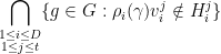
 from a finite subset of
  and
and 
 , there exists
 ,
,  ,
,  with
with
 is
is 

 .
. and the dominated hyperplane
  for the actions of the proximal matrices
  on
on  , say
, say  , such that
 .
. is attracted towards
  . By rendering this argument slightly more quantitative (with the aid of the so-called Tits proximality criterion), Breuillard and Sert proved in
  is
is  is a finite subset such that
 and
and  such that for all
  and
and  is
is  -proximal for all
  .
. , we can select
  is
is  .
.

 with
with 
 and
and

 .
. as
as  .
. and a constant
  such that for all
  with
with  and
and

 , we have that
  is bounded and, a fortiori,
 , as desired.
  with
with  is realized by a single sequence
  in the sense that
  .
. with the property that
  is a Schottky family in the sense that
  is
is  and
and  for all
  where
where  .
. so that
 by
by
 has the form
  where
where  and
and  is a prefix of
  . Observe that
 . Moreover,
  makes that
  is a
is a  -proximal element with
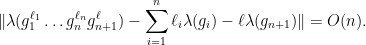
 converges to
  converges to
  -plane can be written as the sum of three terms; for the
  -norm of Beltrami differentials with essentially disjoint supports; finally, this
  , and we dispose of good upper bounds for
  and all of its derivatives in terms of the distance of
  using the techniques of these articles
  are small whenever
  is a polynomial function on
 ![{[0,1]}](https://s0.wp.com/latex.php?latex=%7B%5B0%2C1%5D%7D&bg=ffffff&fg=000000&s=0&c=20201002) whose degree and
whose degree and  and
and  with
with  , there exists a constant
  with the following property.If
  denotes the product of the lengths of the short geodesics of a hyperbolic surface
 .
. with
with  . If we write
  , where
  is the usual hyperbolic plane and
  of Riemann surfaces of genus
  of harmonic
  induced by the Hermitian inner product
 and
and  is the hyperbolic area form on
  and
and  are Beltrami differentials, then
  is a function on
 and
and  is an operator related to the
  on
on  .
. .
. and
and  span a
  and
and  such that
  ,
,  , and
, and  is orthonormal. Then, Bochner showed that the

 is a positive operator on
  with unit norm. Finally,

 . (Here,
  stands for the hyperbolic distance on
  and
and  whenever
 of a
of a 
 into its real and imaginary parts, say
  , then we see that
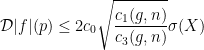
![\displaystyle \begin{array}{rcl} \textrm{Re}(1\overline{2}, 1\overline{2}) - (1\overline{2}, 2\overline{1}) &=& \left[\int_X f\,\mathcal{D}f \, dA - \int_X h\, \mathcal{D}h \, dA\right] - \left[\int_X f\,\mathcal{D}f \, dA + \int_X h\, \mathcal{D}h \, dA\right] \\ &=& -2\int_X h\, \mathcal{D}h \, dA. \end{array}](https://s0.wp.com/latex.php?latex=%5Cdisplaystyle+%5Cbegin%7Barray%7D%7Brcl%7D+%5Ctextrm%7BRe%7D%281%5Coverline%7B2%7D%2C+1%5Coverline%7B2%7D%29+-+%281%5Coverline%7B2%7D%2C+2%5Coverline%7B1%7D%29+%26%3D%26+%5Cleft%5B%5Cint_X+f%5C%2C%5Cmathcal%7BD%7Df+%5C%2C+dA+-+%5Cint_X+h%5C%2C+%5Cmathcal%7BD%7Dh+%5C%2C+dA%5Cright%5D+-+%5Cleft%5B%5Cint_X+f%5C%2C%5Cmathcal%7BD%7Df+%5C%2C+dA+%2B+%5Cint_X+h%5C%2C+%5Cmathcal%7BD%7Dh+%5C%2C+dA%5Cright%5D+%5C%5C+%26%3D%26+-2%5Cint_X+h%5C%2C+%5Cmathcal%7BD%7Dh+%5C%2C+dA.+%5Cend%7Barray%7D+&bg=ffffff&fg=000000&s=0&c=20201002)
 and, a fortiori,
 . Therefore,


 , so that it follows from
  .
. at this stage: indeed,
  would force a case of equality in Cauchy-Schwarz inequality and this is not possible in our context because
  for the Lyapunov exponents of the Teichmüller geodesic flow. In fact, after some computations with variational formulas for the so-called Hodge norm, Forni establishes that
  and
and  with the following property. If we have an almost equality
 and
and  in
in  and
and 
 [implied by
  . In order to illustrate this point, let us now show Theorem
  such that
 do not belong to the cusp region
  of
of  (equipped with the hyperbolic metric
  ).
). , before explaining the extra ingredient needed to treat the general case.
 for a constant
  to be chosen later. In this regime, our goal is to show that
  is “small”, so that
  is necessarily “big”.
 (cf.
(cf.  (where
  and
and  are the positive and negative parts of the real part
  , then we obtain that
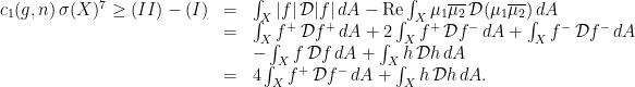
 . Thus, if
 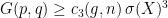 for all
  . It follows that
 , i.e.,
  . By plugging this information into the previous inequality, we obtain the estimate
 (cf.
(cf. 
 for
for  . Since
  for
for 

 bound on
  can be converted into a
  and replacing Beltrami differentials
  and
and  (namely, quadratic differentials), we are led to study quartic differentials
  . By Cauchy integral formula on
 and the cusp region
  is
is  . Thus, there exists an universal constant
  such that
 , we have that the previous inequality implies the following
  :
:


 . This proves Theorem
 is chosen correctly, then the Cauchy integral formula and the Schwarz lemma can be used to prove that
 .
. and this allows us to repeat the arguments of the case
  ,
,  , etc. without any extra difficulty: see Section 5 of Wolpert’s preprint for more details.
 and
and  (cf. Section
 of a short simple closed geodesic
  .
. in terms of the behaviours of simple geodesic arcs connecting
  be the shortest geodesic connecting
  permits to check that it suffices to study the passages of
  giving a “contribution” to
 depending only on the topology of
  -diffeomorphism
  of the circle
  has a well-defined
  (which can be defined using the cyclic order of its orbits, for instance);
 (i.e.,
  for a surjective continuous map
  ) whenever its rotation number
  has irrational rotation number
  (i.e., there is an homeomorphism
  such that
  );
); for some
  ,
,  , and all
  , then there exists
  conjugating
  such that
  for all
  conjugated to
  . (The nomenclature is motivated by
  , the
, the  g.i.e.t.s
  of restricted Roth type such that
  -submanifold of codimension
  where
where  and
and  intervals.
 , so that
  and also
  . Hence, Marmi–Moussa–Yoccoz theorem says that its local conjugacy class of
  regardless of the differentiability scale
 grows linearly with the differentiability scale
  g.i.e.t.
  are
are  sending a finite partition (modulo zero)
  of
of  into closed subintervals
  disposed accordingly to a bijection
  to a finite partition (modulo zero)
  of
of  disposed accordingly to a bijection
  (via
(via  ), an elementary step of the Rauzy–Veech algorithm produces a new
  by taking the first return map of
  where
where  , resp.
  whenever
  , resp.
  (and
(and  ).
). can be iterated indefinitely. This nomenclature is partly justified by the fact that Yoccoz generalized the proof of Poincaré’s theorem in order to establish that a
  for all
  ,
,  ).
). . By definition, the logarithm
  of the slope of
  taking a constant value
  on each continuity interval
  with bi-infinite
 at a point
  with orbit
  for all
  is defined as
  , resp.
  for
for  .
. for all
  with bi-infinite
  given by the first return map of
  .
. associated to an elementary step
  to a function
  ,
,  , where
  stands for the first return time to
  .
. is constant on each
  whenever
  is constant on each
  . In particular, the restriction of
  . The family of matrices obtained from the successive iterates of the Rauzy–Veech algorithm provides a concrete description of the so-called Kontsevich–Zorich cocycle.
 and
and  of genera
  . Among their several curious features, we would like to point out that the following fact proved by
  or
or  intervals (resp.) associated to the first return map of the translation flow
  ,
,  and a
and a  -dimensional vector subspace
  such that
  is an equivariant decomposition with respect to the matrices of the Kontsevich–Zorich cocycle with the following properties:
 ;
; ;
; are usually called the tautological exponents of the Kontsevich–Zorich cocycle. In this terminology, the third item above is saying that all non-tautological Lyapunov exponents of the Kontsevich–Zorich associated to
  of
of  (see, e.g., Section 3.4 of
  under the Rauzy–Veech algorithm actually coincides with
  , then the item (c) from Subsection
  for all
  and this allows to select a bounded subsequence of
  thanks to the repetition of certain words in the prefix-suffix decomposition.
 such that
  , when
  always lead to piecewise affine i.e.t.s which are not
  for some
 is a
is a  is a solution of the
  are bounded and, by continuity of
  of
of  belongs to the weak stable space of the Kontsevich–Zorich cocycle (compare with Remark 3.9 of Marmi–Moussa–Yoccoz paper).
Recent Comments