Today we’ll close our current discussion of the standard map with the proof of Duarte’s theorem. As we mentioned earlier, the basic strategy consists into three steps: the construction of a dynamically increasing family of hyperbolic basic sets of saddle-type (“horseshoes”), the existence of a dense set of parameters where a quadratic tangency is generically unfolded and the construction of elliptic islands from the bifurcation of quadratic tangencies via a conservative version of Newhouse phenomena. More precisely, we are going to show the statements of theorems 1, 2 and 3 of the previous post.
–An “increasing” family of hyperbolic basic sets–
In order to find hyperbolic sets, we’ll use the well-known invariant cone-field criterion:
Theorem (invariant cone-field criterion). Let  be a
be a  -diffeomorphism. Consider
  a compact
  -invariant set. Assume that there are
  , a decomposition
  (not necessarily
  -invariant) and two families
  ,
,  of (closed) cones such that
 and
and  for all
  and
and  ;
; and
and  for all and
  .
.
Then, is a hyperbolic set.
Proof. See corollary 6.4.8 of Katok-Hasselblat book. A sketch of proof goes as follows. Fix a point and consider the following two sequences of cones on the tangent space  :
:  and
and  . Our assumptions implies that these two sequences are nested sequences of closed cones, so that the intersections
and
are closed –invariant closed cones. In fact, one can work a bit more (with the facts and ) to see that  and
and  are vector subspaces with dimensions
  and
and  resp.. Finally, once we know that and are -invariant subspaces, our assumptions of expansion (resp. contraction) of vectors belonging to the cone
  (resp.
  ), we see that is the unstable subspace and is the stable subspace. This completes the sketch.
Proposition 1. Consider the invertible area-preserving map

of the 2-torus  and let be a -invariant compact set. Assume that there exists
  such that
  for all
  . Then, is a hyperbolic set (of saddle type).
Proof. Note that

In particular, the trace of verifies  so that the matrices are uniformly hyperbolic. In fact, this follows from the fact that the constant cone-field

is an unstable cone-field whenever  (note that such a choice is possible since ). Indeed, if we write
  , we see that

so that  where
where  by the choice of the parameter
  , i.e.,
  is -invariant. Furthermore, denoting by
  , we get, for any
  ,
,

with  , i.e., (uniformly) expands any vector inside
  . On the other hand, it is not hard to see that
  implies that the same argument can be applied to
  in order to get a stable cone-field. Using the invariant cone-field criterion, the proof is complete.
An immediate consequence of this proposition is the following result:
Corollary 1. For the standard family
 ,
,
given any , the maximal invariant set
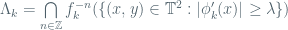
is hyperbolic.
Remark. It is worth to note that this result gives a clue about the location of the critical region of non-hyperbolicity: for a given , the set of points  converges to the union of the two circles
  when
when  .
.
Of course, this corollary says that the hyperbolic sets  are a family of dynamically increasing basic sets. In fact, it turns out that this can be checked by hand (see section 4.2 of Duarte’s paper), but we’ll skip this fact for sake of brevity of the exposition.
–Global dynamical foliations and their tangency lines–
After the description of the (“big”) hyperbolic sets of the standard map  , we proceed to the study of the tangencies between their invariant foliations. In order to do so, we need to extend these foliations to some uniform neighborhood of (since we want to perform an analysis for several large parameters) while keeping good estimates of distortion of the holonomy maps. At this point, our first technical problem arises: from the general theory of uniformly hyperbolic sets (see the book of Palis-Takens), we know that admits some neighborhood
  so that the stable and unstable foliations of can be extended to (while keeping good estimates), but a priori the region where the good estimates are ensured can deteriorate when . To overcome this problem, Duarte takes the following point of view. Near the critical region , he replaces
  by a function
  having two poles at
  and he tries to compare the dynamics of
  with the dynamics of the singular diffeomorphism
  .
.
More precisely,  where
where  outside a
  -neighborhood of and
  . Then, after the somewhat tedious work of redoing the theory of invariant manifolds (following the exposition of Hirsch-Pugh-Shub), he checks that
  has global stable and unstable foliations
  on
on  verifying uniform distortion estimates (i.e., their holonomy maps have uniformly bounded
  -norm). Here, the uniform control of distortion comes from the choice of
  : indeed, assuming that coincides with
  outside a
  -neighborhood of , it is not hard to see that the Schwartzian derivate of is bounded from below (in the critical region
  ) by
) by
 .
.
In particular, since we want to take  the largest possible so that coincides with in
  and with bounded Schwartzian derivative (because it is well-known that bounded Schwartzian derivative implies bounded distortion), it is natural to take
  outside
  (i.e.,
  ).
).
Of course, once we performed this work (which takes 21 pages of Duarte’s paper), we have to compare the dynamics of and  . However, this is not hard: the maximal invariant set is the same for both and , and, using the strong hyperbolic features of the singular diffeomorphism , it is possible to show that the dynamics of and on are conjugated to a
  full (Bernoulli) shift (where
  ); furthermore,
  , its stable and unstable thickness
  (where
  , resp.
  , is the thickness of the Cantor set obtained by projection of along the stable, resp. unstable, foliation on an arbitrarily fixed transversal section) and, as a consequence, its Hausdorff dimension
  satisfies
  .
.
Next, we analyse the relative positions of the (-invariant) foliations  and
and  . Applying to , we obtain a new foliation
  (recall that is -invariant but it is not -invariant). It is not hard to see that the set of tangencies between
  and are two circles close to . Moreover, the projection of along and
  into these two circles gives rise to two Cantor sets
  and
and  satisfying
  and
and  (here we are using the previous thickness estimate and the fact that the application of to the foliation doesn’t change very much the thickness). The picture below (borrowed from Duarte’s paper) summarizes our discussion about the relative position of and :
 Here is the almost vertical foliation and is the foliation folding along the two dotted circles. Now, using the fact that
  (for any large
  ), we can apply Newhouse’s gap lemma to obtain that
  . In other words, we get that and exhibits persistent tangencies.
Remark. In proposition 16 of Duarte’s paper, a version of Newhouse’s gap lemma in the circle is wrongly stated: indeed, Duarte claims that the fact that the two Cantor sets are contained in the circle automatically implies that the two Cantor sets are linked. However, this is not correct (as the example of two thick Cantor sets supported by two disjoint compact intervals shows), although this is not a serious problem for this argument: from a careful checking of the geometry of (via the features of the singular diffeomorphism ), it is not hard to see that and are linked (this follows from Duarte’s argument in section 4.2 of his paper).
Finally, closing this section, we claim that these persistent tangencies are quadratic and unfold generically with the parameter (as the picture above indicates). While a complete proof of this result takes 7 pages of technical calculations, we’ll provide a convincingly enough (I hope! :)) heuristic argument. We know that the -invariant foliations and are almost vertical and horizontal (resp.). In particular, it is reasonable to expect that the circles of tangencies between and  are close to the circles of tangencies between the horizontal foliation and the image of the vertical foliation under . On the other hand, since
  where
where  is the
  counterclockwise rotation and
  is a shear (of variable intensity) along the horizontal foliation, we can compute the image of the vertical foliation under as follows: the image of the horizontal foliation by
  is the vertical foliation and the image of the vertical foliation by
  is a foliation by the family of curves which are parallel to the graph
  . In particular, the circle of tangencies between these two foliations are exactly the critical circles
  . At such points, the difference between the curvatures is measured by
  , so that the tangencies between the horizontal foliation and the -image of the vertical foliation are quadratic (i.e., locally you are seeing the intersections between straight lines and parabolas) and, a fortiori, the same holds for the tangencies between and . Also, when the parameter increases, the -invariant foliations and doesn’t change very much (they are almost constant), while the
  -coordinates of the tangency points between
  and (which are close to
  ) move with velocity (close to) 1 (indeed,
  implies
  ). Hence, these tangencies are unfolded generically.
At this point, the reader noticed that this discussion gives the theorems 1 and 2 of the previous post. Now, we proceed to discuss the conservative version of the Newhouse phenomena.
-Conservative version of Newhouse phenomena: proof of theorem 3-
Before entering into the proof of the abundance of elliptic islands close to a generically unfolded quadratic tangency, let me review a little bit some facts around the proof of the “classical” Newhouse phenomena.
Given  a 1-parameter family of surface diffeomorphisms generically unfolding a quadratic homoclinic tangency
  associated to a hyperbolic periodic point
  of saddle-type (at the parameter
  say), Newhouse manage to define a renormalization scheme near as follows: for every large
  , one can select small boxes near which are mapped by
  near itself with the shape of a parabola so that their relative positions resembles a horseshoe; next, we compose this dynamics with appropriate rescalings
  of these boxes in order to put these very small boxes into a fixed scale (e.g., a unit square) so that we obtain the families of dynamical systems given by
  (these are called the successive renormalizations of the dynamics near the homoclinic tangency). The usefulness of idea is more or less clear: assuming that there exists some limiting object
  , any stable dynamical property of
  will be shared by
  and a fortiori . It turns out that Newhouse showed that this renormalization scheme converges (i.e., the limiting object exists) when the periodic point is dissipative (i.e.,
  ). Moreover, the limit in this case is the quadratic family
 .
.
Using this information, the existence of sinks near the homoclinic tangency follows directly. A detailed exposition of Newhouse’s argument can be found in the excelent book of Palis and Takens.
After this quick review of Newhouse arguments, let us consider again the situation of the standard map: in the conservative setting, given a family of area-preserving diffeomorphisms generically unfolding a quadratic homoclinic tangency associated to a hyperbolic periodic point, one can repeat the renormalization scheme of Newhouse to get as a limit object the conservative Hénon family
 .
.
Next, it is possible (exercise) to show the presence of elliptic fixed points for this family when  (with the eigenvalue of this point running from 1 to -1). Because generic (i.e., non-resonant) elliptic periodic point is stable by conservative perturbations (this follows from the so-called KAM theory; see e.g. this monograph of J. Moser), we conclude the existence of (generic) elliptic periodic points nearby the homoclinic tangency. Combining this result with the theorems 1 and 2 proved in the previous sections, we see that, similarly to the proof of Newhouse theorem, the proof of theorem 3 is complete!

Leave a comment