On the continuity of Lyapunov spectrum for random products

Posted by: matheuscmss | February 5, 2014

On the continuity of Lyapunov spectrum for random products

Last week, the conference “Random walks on groups” took place at IHP as part of the activities of a trimester on random walks and asymptotic geometry of groups (organized by Indira Chatterji, Anna Erschler, Vadim Kaimanovich, and Laurent Saloff-Coste) from January to March 2014.

Given the very interesting program of this conference, it was not surprising that Amphithéâtre Hermite (where the talks were delivered) was always full.

Today, we will discuss one of the talks of this conference, namely, the talk “On the continuity of Lyapunov spectrum for random products” of Alex Eskin about his joint work (in preparation) with Artur Avila and Marcelo Viana.

As usual, all mistakes/errors in this post are entirely my responsibility.

Remark 1 A video of a talk of Artur Avila on the same subject can be found here.

Update [February 11, 2014]: Last Friday, I was lucky enough to get some extra explanations concerning “costs of couplings” directly from Alex. At the end of this post (see the “Epilogue”), I will try to briefly summarize what I could understand from this conversation.

1. Introduction

Let ${\mu}$ be a probability measure on ${SL(d,\mathbb{R})}$ , e.g., ${\mu=\sum\limits_{i=1}^{n}p_i\delta_{A_i}}$ where ${(p_1,\dots, p_n)}$ is a (non-trivial) probability vector (i.e., ${\sum\limits_{i=1}^n p_i=1}$ and ${p_i>0}$ for all ${i=1,\dots, n}$ ) and ${\delta_{A_i}}$ are Dirac masses at ${A_i\in SL(d,\mathbb{R})}$ .

Consider the random walk on ${G=SL(d,\mathbb{R})}$ induced by ${\mu}$ , i.e., let ${\Omega=G^{\mathbb{N}}}$ , ${\mathbb{P}=\mu\times\mu\times\dots=\mu^{\mathbb{N}}}$ , and, for each ${n\in\mathbb{N}}$ , ${w=(X_0,\dots, X_k,\dots)\in\Omega}$ , put

$\displaystyle A(n,w):=X_n\dots X_0$

Remark 2 Of course, the intuition here is that the samples ${A(n,w)}$ , ${n\in\mathbb{N}}$ , are describing a random walk on ${G}$ whenever we perform a random choice of ${w=(X_0,\dots, X_i,\dots)}$ with respect to ${\mathbb{P}}$ (or, equivalently, random choices of ${X_i}$ ‘s with probability distribution ${\mu}$ ).

In this context, the Oseledets multiplicative ergodic theorem says that:

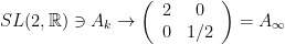
Theorem 1 (Oseledets) For ${\mathbb{P}}$ -almost every ${w\in\Omega}$ , one has

$\displaystyle [A(n,w)^T A(n,w)]^{\frac{1}{2n}}\rightarrow\Lambda$

where ${\Lambda}$ is a symmetric matrix with eigenvalues ${e^{\lambda_1}\geq\dots\geq e^{\lambda_d}}$ . (Here, ${A^T}$ is the transpose matrix of ${A\in G}$ , and ${B=[A^TA]^{\frac{1}{2n}}}$ denotes the non-negative symmetric matrix such that ${B^{2n}=A^TA}$ .)

The numbers ${\lambda_1\geq\dots\geq\lambda_d}$ are called Lyapunov exponents.

Geometrically, Oseledets theorem says that the random walk ${A(n,w)}$ almost surely tracks a geodesic of speed ${\sqrt{\lambda_1^2+\dots+\lambda_d^2}}$ of the symmetric space ${G/K}$ (where ${K=SO(d,\mathbb{R})}$ is a maximal compact subgroup of ${G}$ ).

Remark 3 The top Lyapunov exponent ${\lambda_1}$ can be recovered by the formula

$\displaystyle \lambda_1=\lim\limits_{n\rightarrow\infty}\frac{1}{n}\log\|A(n,w)\|$

for ${\mathbb{P}}$ -a.e. ${w}$ , and the remaining Lyapunov exponents can be recovered by the following standard trick/observation: the top Lyapunov exponent of the action of ${SL(d,\mathbb{R})}$ on the ${k}$ -th exterior power ${\wedge^k\mathbb{R}^d}$ is ${\lambda_1+\dots+\lambda_k}$ . For this reason, it is often (but not always!) the case that the results about the top Lyapunov exponent also provide information about all Lyapunov exponents.

Historically, the first results about the Lyapunov exponents of random products ${A(n,w)}$ concerned their multiplicities for a fixed probability distribution ${\mu}$ . A prototypical theorem in this direction is the following result of Guivarch-Raugi and Goldsheid-Margulis providing sufficient conditions for the simplicity (multiplicity ${1}$ ) of Lyapunov exponents.

Definition 2 We say that ${\mu}$ is not strongly irreducible whenever there exists a finite collection ${V_1,\dots, V_k}$ of subspaces of ${\mathbb{R}^d}$ such that

$\displaystyle g(V_1)\cup\dots\cup g(V_k)=V_1\cup\dots\cup V_k$

for all ${g\in\textrm{supp}(\mu)}$ .

Definition 3 We say that ${\mu}$ is proximal if there exists ${g\in\langle\textrm{supp}(\mu)\rangle^{\textrm{Zariski}}}$ such that ${g^T g}$ has distinct eigenvalues. (Here, ${\langle H\rangle^{\textrm{Zariski}}}$ is the Zariski closure of the group generated by ${H\subset G=SL(d,\mathbb{R})}$ .)

Remark 4 If ${\textrm{supp}(\mu)}$ is Zariski dense in ${G=SL(d,\mathbb{R})}$ , then ${\mu}$ is strongly irreducible and proximal.

Theorem 4 (Guivarch-Raugi, Goldstein-Margulis)

1) If ${\mu}$ is strongly irreducible and proximal, then ${\lambda_1>\lambda_2}$ (i.e., the top Lyapunov exponent is simple/has multiplicity ${1}$ );

2) If ${\textrm{supp}(\mu)}$ is Zariski dense in ${SL(d,\mathbb{R})}$ , then ${\lambda_1>\lambda_2>\dots>\lambda_d}$ .

2. Statement of the main result

In their work, Avila, Eskin and Viana consider how the Lyapunov exponents change when the probability distribution varies. Among the results that they will prove in their forthcoming article is:

Theorem 5 (Avila-Eskin-Viana) Suppose ${(p_1,\dots, p_n)}$ is a fixed probability vector, and consider the probability measures

$\displaystyle \mu=\sum\limits_{i=1}^n p_i\delta_{A_i}$

whose support ${A_1,\dots, A_n\in G=SL(d,\mathbb{R})}$ varies. Then, for each ${j=1,\dots, d}$ , the Lyapunov exponent ${\lambda_j}$ is a continuous function of ${A_1,\dots, A_n}$ .

Remark 5 This statement looks innocent, but it is known that Lyapunov exponents do not vary continuously (only upper semi-continuously) “in general”. See, e.g., this article of Bochi (and the references therein) for more details.

3. Previous works and related results

The theorem of Avila-Eskin-Viana generalizes to any dimension ${d\geq 2}$ the work of Bocker-Neto and Viana in dimension ${2}$ :

Theorem 6 (Bocker-Neto-Viana) For a fixed probability vector ${(p_1,\dots, p_n)}$ , the two Lyapunov exponents of

$\displaystyle \mu=\sum\limits_{i=1}^n p_i\delta_{A_i}$

depend continuously on ${A_1,\dots, A_n\in SL(2,\mathbb{R})}$ .

On the other hand, if one decides to fix the support ${A_1,\dots, A_n}$ and to vary the vector of probabilities, then Peres showed in 1991 that:

Theorem 7 (Peres) Let us fix the support ${A_1, \dots, A_n\in SL(d,\mathbb{R})}$ . Then, the simple Lyapunov exponents of

$\displaystyle \mu=\sum\limits_{i=1}^n p_i\delta_{A_i}$

are locally real-analytic function of ${(p_1,\dots,p_n)}$ . More precisely, given ${1\leq j\leq d}$ and a probability vector ${(p_1^{0},\dots, p_n^{(0)})}$ such that the ${j}$ th Lyapunov exponent is simple (i.e., multiplicity ${1}$ ), then the ${j}$ th Lyapunov exponent is a real-analytic function of ${(p_1,\dots,p_n)}$ near ${(p_1^{(0)},\dots, p_n^{(0)})}$ .

The formula 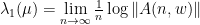${\lambda_1(\mu)=\lim\limits_{n\rightarrow\infty}\frac{1}{n}\log\|A(n,w)\|}$ for ${\mathbb{P}}$ -a.e. ${w}$ for the top Lyapunov exponent is not very useful to study how Lyapunov exponents vary with ${\mu}$ because the notion of “ ${\mathbb{P}}$ -a.e. ${w}$ ” changes radically with ${\mu}$ .

A slightly more useful formula was found by Furstenberg:

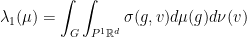
$\displaystyle \lambda_1(\mu)=\int_{G}\int_{P^1\mathbb{R}^d}\sigma(g,v)d\mu(g)d\nu(v)$

where ${\sigma(g,v)=\frac{\|gv\|}{\|v\|}}$ and ${\nu}$ is a ${\mu}$ -stationary measure (i.e., ${\nu}$ is invariant in average with respect to ${\mu}$ , that is, ${\mu\ast\nu:=\int_G g_*\nu d\mu(g)=\nu}$ ) on the projective space ${P^1\mathbb{R}^d}$ of lines in ${\mathbb{R}^d}$ .

Of course, the cocycle ${\sigma(g,v)}$ depends nicely on ${g}$ and ${v}$ , but the dependence on ${\mu}$ of the stationary measure ${\nu}$ in Furstenberg’s formula is not obvious to determine. In particular, one needs to “feed” Furstenberg’s formula with extra information in order to deduce continuity of the top Lyapunov exponent in a given setting.

For example, if one feeds the following remark

Remark 6 If ${\mu}$ is strongly irreducible and proximal, then the stationary measure ${\nu}$ on ${P^1\mathbb{R}^d}$ is unique.

to Furstenberg’s formula, then one can deduce:

Proposition 8 Suppose ${\mu_k\rightarrow\mu_{\infty}}$ (in the weak-* topology), ${\mu_{\infty}}$ is proximal and strongly irreducible. Then, ${\lambda_1(\mu_k)\rightarrow\lambda_1(\mu_{\infty})}$ .

Proof: Denote by ${\nu_k}$ the sequence of stationary measures associated to ${\mu_k}$ in Furstenberg’s formula. It is not hard to check that any accumulation ${\eta_{\infty}}$ of the sequence ${\nu_k}$ is ${\mu_{\infty}}$ -stationary. By the previous remark, ${\mu_{\infty}}$ has an unique stationary measure on ${P^1\mathbb{R}^d}$ , so that any accumulation ${\eta_{\infty}}$ of ${\nu_k}$ coincides with the stationary measure ${\nu_{\infty}}$ in Furstenberg’s formula for ${\mu_{\infty}}$ . In other words, ${\nu_k\rightarrow\nu_{\infty}}$ , and the desired proposition now follows immediately from Furstenberg’s formula. $\Box$

Remark 7 Le Page showed that the conclusion of the previous proposition can be improved from continuity to real-analyticity. However, in general (without strong irreducibility and proximality of ${\mu_{\infty}}$ ), one can not expect anything better than Hölder continuity.

4. Some ideas of the proof of Avila-Eskin-Viana theorem

Let us simplify the exposition by considering the following toy case: we are given two sequences of matrices

$\displaystyle SL(2,\mathbb{R})\ni A_k\rightarrow\left(\begin{array}{cc}2&0\\ 0&1/2\end{array}\right)=A_{\infty}$

and

$\displaystyle SL(2,\mathbb{R})\ni B_k\rightarrow\left(\begin{array}{cc}1/2&0 \\ 0&2\end{array}\right)=B_{\infty}$

and we want to show that the top Lyapunov exponents of the probabilities

$\displaystyle \mu_k=\frac{2}{3}\delta_{A_k}+\frac{1}{3}\delta_{B_k}$

converge to

$\displaystyle \lambda_1(\mu_k)\rightarrow\frac{2}{3}\log2+\frac{1}{3}\log(1/2)=\frac{1}{3}\log2=\lambda_1(\mu_{\infty})$

The projective actions of the matrices ${A_{\infty}}$ and ${B_{\infty}}$ on the projective circle ${P^1\mathbb{R}^2=S^1}$ are of “north pole–south pole type”: there are two fixed points ${p_+}$ and ${p_-}$ corresponding to the directions of the coordinate axes ${x}$ and ${y}$ of ${\mathbb{R}^2}$ and the points of ${P^1\mathbb{R}^2}$ are either attracted or repelled towards ${p_+}$ and ${p_-}$ under the actions of ${A_{\infty}}$ and ${B_{\infty}}$ . In particular, one can infer from this that an arbitrary ${\mu_{\infty}}$ -stationary measure on ${P^1\mathbb{R}^2}$ has the form

$\displaystyle a\delta_{p_+}+b\delta_{p_-}$

with ${a+b=1}$ .

Therefore, if we denote by ${\nu_k}$ the ${\mu_k}$ -stationary measures coming from Furstenberg’s formula, then

$\displaystyle \nu_k\rightarrow c_+\delta_{p_+}+c_-\delta_{p_-}$

and our goal is to show that ${c_-=0}$ . However, there is not so easy as it seems (in the sense that naive methods don’t work well) and one has to look for appropriate tools.

In this direction, the notion of Margulis function comes at hand. Given a probability measure ${\mu}$ on a group ${G}$ acting on a space ${X}$ , let

$\displaystyle A_{\mu}(f)(x):=\int_G f(gx)d\mu(g)$

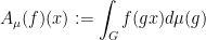
be the Markov operator associated to ${\mu}$ . We say that ${f:X\rightarrow\mathbb{R}}$ is a Margulis function if:

1) ${f\geq 0}$
2) ${f=+\infty}$ on a “negligible set” ${N\subset X}$
3) there are constants ${0<c<1}$ and ${0\leq b<\infty}$ such that ${(A_{\mu})f(x)\leq cf(x)+b}$ , i.e., when ${f}$ is large at a point (a step of a ${\mu}$ -random walk approaches ${N}$ ), the value of ${f}$ at the ${G}$ -images of this point decrease in average (the next step of a ${\mu}$ -random walk tend to get far from ${N}$ ).

Coming back to toy case, it is possible to show that for ${0<\delta\ll1}$ the function ${f:S^1\rightarrow\mathbb{R}}$ given by

$\displaystyle f(x)=\frac{1}{d(x,p_-)^{\delta}}$

is a Margulis function for ${\mu_{\infty}}$ .

This type of information is useful to show simplicity of the Lyapunov exponents of ${\mu_{\infty}}$ , but it does not help us to show the continuity statement ${\lambda_1(\mu_k)\rightarrow \lambda_1(\mu_{\infty})}$ or ${c_-=0}$ . In fact, the difficulty comes from the fact that ${f}$ is not a Margulis function of ${\mu_k}$ because the south pole of ${\mu_k}$ is changing location (even though they are close to ${p_-}$ ), so that a single Margulis function is not capable of assigning the value ${\infty}$ to all of the south poles of ${\mu_k}$ without being trivial.

Here, one can try to overcome the technical obstacle of the moving south poles of ${\mu_k}$ by considering the diagonal action of ${G=SL(2,\mathbb{R})}$ on ${S^1\times S^1}$ and by introducing the function

$\displaystyle f(x,y)=\frac{1}{d(x,y)^{\delta}}$

for ${x}$ and ${y}$ close to ${p_-}$ . As it turns out, this function is a good candidate of Margulis function for ${\mu_k}$ in the sense that the inequality in item 3) involving the Markov operator is satisfied near ${(p_-,p_-)}$ , and it seems that we are doing some progress.

Unfortunately, we made no progress at all with the idea in the previous paragraph: indeed, the technology of Margulis functions requires globally defined functions and so far we were able only to exhibit locally defined functions (in a neighborhood of ${(p_-,p_-)}$ ).

At this point, the basic idea of Avila-Eskin-Viana is the introduction of measure-theoretical analogs of Margulis functions. In other terms, they want to replace “functions” by “measures” to get objects that are slightly more flexible but still capable of doing the same job than Margulis functions.

The measure-theoretical analog of Margulis functions are called couplings with finite costs. Concretely, we say that a probability measure ${\eta_k}$ on ${S^1\times S^1}$ is a coupling of ${\nu_k}$ to itself if the projection of ${\eta_k}$ to both factors is ${\nu_k}$ . Given a coupling ${\eta_k}$ of ${\nu_k}$ to itself, we define its cost as:

$\displaystyle \textrm{cost}(\eta_k)=\int_{U_-\times U_-}\frac{1}{d(x,y)^{\delta}}d\eta_k(x,y)$

where ${U_-}$ is an adequate small neighborhood of ${p_-}$ .

In this setting, we can see that the task of showing ${c_-=0}$ is reduced to find a large constant ${C}$ and a sequence of couplings ${\eta_k}$ of ${\nu_k}$ to itself such that

$\displaystyle \textrm{cost}(\eta_k)<C$

for all ${k\in\mathbb{N}}$ . Indeed, this is so because the cost of coupling ${\delta_{p_-}}$ to itself is ${\infty}$ and thus ${c_+\delta_{p_+}+c_-\delta_{p_-}}$ has finite cost only when ${c_-=0}$ .

At this point, the time of Alex Eskin was essentially out and he concluded by saying that the main point is that finding couplings with finite costs is easier than building globally defined Margulis functions, and the desired couplings ${\eta_k}$ with uniformly bounded costs could be found by analyzing the analog of item 3) in the definition of Margulis functions for couplings of ${\nu_k}$ to itself with optimal (minimal possible) costs.

5. Epilogue

Let us try to give more explanations to the discussion in the previous 6 paragraphs above (following my conversation with Alex Eskin [or what I can remember of it…]).

We start by selecting the small neighborhood $U_-$ of $p_-$ so that the limit stationary measure $\nu_{\infty}$ gives mass

$0.99\nu_{\infty}(U_-)\leq\nu_{\infty}(\{p_-\})$

to $U_-$ .

Then, we restrict our measures $\nu_k$ to $U_-$ and we change the dynamics so that these restrictions are stationary: formally, we replace the Markov operator $A_{\mu_k}$ by an adequate “local transfer operator” $T_{\mu_k}:L^{\infty}(U_-)\to L^{\infty}(U_-)$ such that $\nu_k|_{U_-}$ is $T_{\mu_k}$ -stationary.

In these terms, the “local version”

$f(x,y)=\left\{\begin{array}{cc}0 & \textrm{ if }x,y\notin U_- \\ \frac{1}{d(x,y)^{\delta}} & \textrm{ otherwise}\end{array}\right.$

of the “usual candidate to Margulis function” $1/d(x,y)^{\delta}$ seems to be a Margulis function at first sight, but unfortunately it does not satisfies item 3). Indeed, the pointwise estimates of the form

$T_{\mu_k}f(x,y)\leq cf(x,y)+b$

with $0<c<1$ and $0<b<\infty$ do not hold always because there are some couples of points $(x,y)$ that are pushed together towards $p_-$ despite the fact that the probability of this event is small.

For this reason, Avila-Eskin-Viana replace “functions” by “measures” with the idea that this probabilistic tendency felt by most couples $(x,y)$ of getting away from $p_-$ is better expressed as estimates for measures than pointwise estimates for functions.

More concretely, by selecting an appropriate subinterval $p_-\in U_{--}\subset U_-$ , one can see that the $\mu$ -measure of the set

$S_x=\{g\in SL(2,\mathbb{R}): gx\in U_{--}\}$

of elements of $SL(2,\mathbb{R})$ pushing a point $x\in U_- - U_{--}$ towards $p_-$ is $\mu(S_x)<1/2$ . From this information, it is not difficult to construct some measures $\widehat{\eta}_{x,y}$ on $SL(2,\mathbb{R})\times SL(2,\mathbb{R})$ such that $\widehat{\eta}_{x,y}$ projects to $\mu$ on both factors and $\widehat{\eta}_{x,y}(S_x\times S_y)=0$ . From the measures $\widehat{\eta}_{x,y}$ , one obtains some couplings $\widehat{\eta}=\widehat{\eta}_k$ with finite costs.

However, this is not quite the end of the history: we need couplings $\eta_k$ whose costs are uniformly bounded for all $k\in\mathbb{N}$ . Here, the trick is to study couplings $\widetilde{\eta}_k$ with optimal costs (i.e. with smallest possible costs). In fact, by applying the “dynamics” $T_k=T_{\mu_k}$ to $\widetilde{\eta}_k$ , one has the following analogue of item 3) in the definition of Margulis functions:

$cost(T_k\widetilde{\eta}_k)\leq c\cdot cost(\widetilde{\eta}_k)+b$

for some universal constants $0<c<1$ and $0<b<\infty$ (thanks to the probabilistic tendency of most couples of points $(x,y)$ to get pushed away from $p_-$ ). On the other hand, since $\widetilde{\eta}_k$ has optimal (smallest) cost, we conclude that

$cost(\widetilde{\eta}_k)\leq cost(T_k\widetilde{\eta}_k)\leq c\cdot cost(\widetilde{\eta}_k)+b,$

that is,

$cost(\widetilde{\eta}_k)\leq b/(1-c)=:C$

In other terms, the analog for measures of item 3) in the definition of Margulis functions allows to check that the costs of the sequence optimal cost couplings $\widetilde{\eta}_k$ are uniformly bounded by $C$ , as desired.

Posted in Conferences, expository, math.DS, Mathematics | Tags: Alex Eskin, coupling with finite cost, couplings of measures, IHP-Paris, Institut Henri Poincare, Lyapunov exponents, Margulis function, random walk, Random Walks and Asymptotic Geometry of Groups

Responses

Dear Professor Matheus
Hi. First of all, i am really thankful because of your nice blog. I have learnt many things from it. I have a question. As far as i know, Avila,Eskin and Viana have annocned which we have proved continuity Lyapunov exponents for arabitary dimension but there is no paper for it. I have been looking for it for some month, even i asked many people, nobody knows about it. Let me know, Do you know, they actully proved it? I know, they gave some talks about their result but after 4, they have not written it. Do you have a preliminary version of their article?
Best regards
Reza
By: Reza on December 21, 2018
at 10:29 am

Reply
- Dear Reza,
  
  As far as I know, you’re absolutely right: the preprint of Avila-Eskin-Viana is not publicly available yet.
  
  Nevertheless, Viana wrote recently a survey (http://w3.impa.br/~viana/out/CS.pdf) containing an exposition of some ideas leading to particular cases of the results claimed by Avila-Eskin-Viana.
  
  Finally, while I don’t have a copy of their preprint, I think you can try to ask one of the authors (say Viana) for a preliminary version of their article.
  
  Best,
  
  Matheus
  By: matheuscmss on December 22, 2018
  at 10:40 am
  
  Reply

M	T	W	T	F	S	S
					1	2
3	4	5	6	7	8	9
10	11	12	13	14	15	16
17	18	19	20	21	22	23
24	25	26	27	28

	Adam on Breuillard-Sert’s joint…
	Adam on Breuillard-Sert’s joint…
	Writing a Hilbert C*… on ERT16: Compact extensions
	matheuscmss on Yoccoz book collection at…
	Jairo B. on Yoccoz book collection at…

Disquisitiones Mathematicae