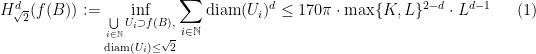
Some of the partial advances obtained by Jacob Palis, Jean-Christophe Yoccoz and myself on the computation of Hausdorff dimensions of stable and unstable sets of non-uniformly hyperbolic horseshoes (announced in this blog post here and this survey article here) are based on the following lemma:
Lemma 1 Let
be a
diffeomorphism from the closed unit ball
of
into its image.Let
and
be two constants such that
and
for all
.
Then, for each
, the
-dimensional Hausdorff measure
at scale
of
satisfies
Remark 1 In fact, this is not the version of the lemma used in practice by Palis, Yoccoz and myself. Indeed, for our purposes, we need the estimate
where
is the ball of radius
centered at the origin and
is a
and
for
. Of course, this estimate is deduced from the lemma above by scaling, i.e., by applying the lemma to
where
is the scaling
.

Nevertheless, we are not completely sure if we should write down an article just with our current partial results on non-uniformly hyperbolic horseshoes because our feeling is that these results can be significantly improved by the following heuristic reason.
In a certain sense, Lemma 1 says that one of the “worst” cases (where the estimate (1) becomes “sharp” [modulo the multiplicative factor 


![{[-\sqrt{\frac{1}{2}}, \sqrt{\frac{1}{2}}]\times [-\sqrt{\frac{1}{2}}, \sqrt{\frac{1}{2}}]\subset B\subset [-1,1]\times [-1,1]}](https://s0.wp.com/latex.php?latex=%7B%5B-%5Csqrt%7B%5Cfrac%7B1%7D%7B2%7D%7D%2C+%5Csqrt%7B%5Cfrac%7B1%7D%7B2%7D%7D%5D%5Ctimes+%5B-%5Csqrt%7B%5Cfrac%7B1%7D%7B2%7D%7D%2C+%5Csqrt%7B%5Cfrac%7B1%7D%7B2%7D%7D%5D%5Csubset+B%5Csubset+%5B-1%2C1%5D%5Ctimes+%5B-1%2C1%5D%7D&bg=ffffff&fg=000000&s=0&c=20201002)


However, in the context of (expectional subsets of stable sets of) non-uniformly hyperbolic horseshoes, we deal with maps
In summary, Jacob, Jean-Christophe and I hope to improve the results announced in this survey here, so that Lemma 1 above will become a “deleted scene” of our forthcoming paper.
On the other hand, this lemma might be useful for other purposes and, for this reason, I will record its (short) proof in this post.
1. Proof of Lemma 1
The proof of (1) is based on the following idea. By studying the intersection of 


Let us now turn to the details of this argument. Denote by 


Consider the following recursively defined cover of 


Next, for each 


In other words, we start with 


Remark 2 In this construction, we are implicitly assuming that
is not entirely contained in a dyadic square
. In fact, if
, then the trivial bound
(for
In this way, we obtain a countable collection 

 .
.By thinking of this expression as a

This reduces our task to estimate these

for any

From this estimate, we see that the
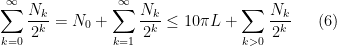
Thus, we have just to estimate the series 

Proof of Claim. Note that 


For the sake of contradiction, suppose that 


- (a) either
is contained in
- (b) or
However, we obtain a contradiction in both cases. Indeed, in case (a), we get that a dyadic square 


a contradiction with the definition of

a contradiction with (2).
This completes the proof of the claim.

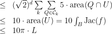
Coming back to the calculation of the series 


By plugging this estimate into (6), we deduce that the

Finally, from (3), (4), (5) and (8), we conclude that

This ends the proof of the lemma.

What kind of diffeomorphisms you have in mind? Can you name an example of a diffeomorphism of the disk where Lemma 1 gives a non-trivial result? In fact, map where I can write the equation or compute
  will be pretty boring. I am not a dynamicist so I can’t think of many examples.
Even though the image is topologially a disk and the boundary is a differentiable, the boundary might be very complicated.
By: MrCactu5 (@MonsieurCactus) on May 11, 2015
at 8:46 pm
A prototype of the kind of diffeomorphisms that we have in mind is defined on a ball
  of doubly exponentially small radius
  (i.e.,
  for some
  ,
,  ) “near” to the origin, where
  is an affine hyperbolic diffeomorphism (with
  and
and  “close” to the origin), and
  is a folding map (given by the composition of a fold
  and a rotation
  ).
).
Here, the point is that is a “complicated” map (algebraic map of degree
  whose coefficients depend on parameters
  ,
,  ), but one can estimate the Hausdorff measure (at scale
  ) of
) of  thanks to (the remark after) Lemma 1.
Indeed, is area-preserving, and, furthermore, one can give a better bound to the derivative of
  than the trivial bound
(where is a bound for the derivative of the folding map
  ) because the derivative of the folding map
  “tends” to send (with some “parabolic” effect) the (horizontal) direction of maximal expansion for
  to (almost vertical) directions of almost maximal contraction for
  , and vice-versa. In particular, by performing the calculation of
  using this observation, one can show that
and this is the one of the important inputs used by Jacob, Jean-Christophe and I in our dynamical applications of the lemma.
I hope this explains why the lemma helps us in this setting (coming from dynamics): we want to estimate the Hausdorff measure (at fixed scale ) of a set
  with complicated geometry (of “algebraic complexity”
  ); instead of looking at the fine details of the geometry of this set, the lemma tells us that one can reasonably estimate the Hausdorff measure (at fixed scale) if there is a “dynamical reason” forcing the derivative and Jacobian of
  to satisfy some better bounds than the “trivial” ones.
In other terms, the lemma gives you good geometrical information (Hausdorff measure, optimal covers of sets) if you dispose of good dynamical/analytical information (non-trivial bounds on derivative and/or Jacobian).
By: matheuscmss on May 12, 2015
at 9:42 am