In a series of two posts, we will revisit our previous discussion on the exponential mixing property for hyperbolic flows via a technique called Dolgopyat’s estimate.
Here, our main goal is to provide a little bit more of details on how this technique works by offering a “guided tour” through Sections 2 and 7 of a paper of Avila-Goüezel-Yoccoz.
For this sake, we organize this short series of posts as follows. In next section, we introduce a prototypical class of semiflows exhibiting exponential mixing. After that, we state the main exponential mixing result of this post (an analog of Theorem 7.3 of Avila-Goüezel-Yoccoz paper) for such semiflows, and we reduce the proof of this mixing property to a Dolgopyat-like estimate on weighted transfer operators. Finally, the next post of the series will be entirely dedicated to sketch the proof of the Dolgopyat-like estimate.
1. Expanding semiflows
Recall that a suspension flow is a semiflow 


Geometrically, 


A more concise way of writing down 


and 

In this post, we want to study the decay of correlations of expanding semiflows, that is, a suspension flow 
Remark 1 Avila-Gouëzel-Yoccoz work in greater generality than the setting of this post: in fact, they allow
to be a John domain and they prove results for excellent hyperbolic semiflows (which are more common in “nature”), but we will always take
and we will study exclusively expanding semiflows (which are obtained from excellent hyperbolic semiflows by taking the “quotient along stable manifolds”) in order to simplify our exposition.
Definition 1 Let
be the Lebesgue measure on
be a finite or countable partition of
is an uniformly expanding Markov map if
is a Markov partition: for each
, the restriction of
is a
-diffeomorphism between
and, for each
such that
for each
;
the inverse of the Jacobian of
the set of inverse branches of
is a
such that
for all
and
. (This condition is also called Renyi condition in the literature.)

Remark 2 Araújo and Melbourne showed recently that, for the purposes of discussing exponential mixing properties (for excellent hyperbolic semiflows with one-dimensional unstable subbundles), the bounded distortion (Renyi condition) can be relaxed: indeed, it suffices to require that
is uniformly bounded for all
Example 1 Let
be the finite partition (mod.
) of
,
. The map
given by
for
An uniformly expanding map 


Indeed, the proof of these facts can be found in Aaronson’s book and it involves the study of the spectral properties of the so-called transfer (Ruelle-Perron-Frobenius) operator

(as it was discussed in Theorem 1 of Section 1 of this post in the case of a finite Markov partition 
Definition 2 Let
is a good roof function if
- there exists a constant
such that
for all
;
- there exists a constant
for all
of
where
is constant on each
is
Remark 3 Intuitively, the condition that
Definition 3 A good roof function
such that
.
The suspension flow 

on 

Remark 4 All integrals in this post are always taken with respect to
unless otherwise specified.
Remark 5 In the sequel, AGY stands for Avila-Gouëzel-Yoccoz.
2. Statement of the exponential mixing result
Let 
Theorem 4 There exist constants
such that
for all
and for all
.

Remark 6 By applying this theorem with
in the place of
, we obtain the classical exponential mixing statement:

Remark 7 This theorem is exactly Theorem 7.3 in AGY paper except that they work with observables
belonging to Banach spaces
and
which are slightly more general than
). In fact, AGY need to deal with these Banach spaces because they use their Theorem 7.3 to deduce a more general result of exponential mixing for excellent hyperbolic semiflows (see their paper for more explanations), but we will not discuss this point here.
The remainder of this post is dedicated to the proof of Theorem 4.
2.1. Reduction of Theorem 4 to Paley-Wiener theorem
From now on, we fix two observables 

Of course, there is no loss in generality here because we can always replace 
In this setting, we want to show that the correlation function

For this sake, we will use the following classical theorem in Harmonic Analysis (stated as Theorem 7.23 in AGY paper):
Theorem 5 (Paley-Wiener) Let
be a bounded measurable function and denote by
(defined for
with
) the Laplace transform of
.Suppose that
can be analytically extended to a function
defined on a strip
in such a way that
Then, there exists a constant
such that
for all
.
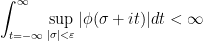

In other words, the Paley-Wiener theorem says that a bounded measurable function decays exponentially whenever its Laplace transform admits a nice analytic extension to a vertical strip to the left of the imaginary axis 
In our context, we will produce such an analytic extension by writing the Laplace transform of the correlation function as an appropriate geometric series of terms depending on 


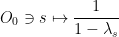
More concretely, for each

where
is the subset of points
whose piece of orbit
hits the graph of the roof function at least once,
- and
is the subset of points
Let us denote by

the corresponding decomposition of the correlation function (3).
The fact that the roof function 

Thus, it is not surprising that the following calculation shows that 

where 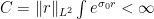
In particular, the proof of Theorem 4 is reduced to show that 

where 
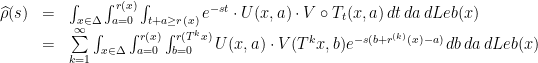
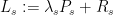
An economical way of writing down this series uses the partial Laplace transform of a function 

By a change of variables 

where 

Remark 8 In general, we expect the terms of the series (4) to decay exponentially because
is “dual” to the (Koopman-von Neumann) operator defined by composing functions with
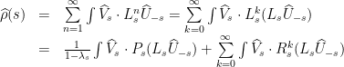
This formula (stated as Lemma 7.17 in AGY paper) is the starting point for the application of Paley-Wiener theorem to
- (a) Lemma 7.21 in AGY paper:
can be extended to a neighborhood of any
;
- (b) Lemma 7.22 in AGY paper:
;
- (c) Corollary 7.20 in AGY paper:
for some
small and
large in such a way that the extension
(for some constant
Geometrically, the first two steps permit to extend

for 

Of course, these steps are not sufficient to extend 

In summary, the combination of the three steps (a), (b) and (c) (and the fact that the function 

Therefore, we have that 
2.2. Implementation of (a), (b) and part of (c)
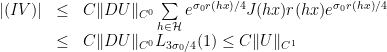
Observe that the series in (4) is bounded by

This hints that we should first compare the sizes of 

Lemma 6 There exists a constant
for any
with
.

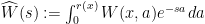
Proof: Recall that 


![\displaystyle \widehat{W}_s(x) = \left[W(x,a)\frac{e^{sa}}{s}\right]_{0}^{r(x)} - \int_0^{r(x)} \partial_a W(x,a) \frac{e^{sa}}{s} \,da](https://s0.wp.com/latex.php?latex=%5Cdisplaystyle+%5Cwidehat%7BW%7D_s%28x%29+%3D+%5Cleft%5BW%28x%2Ca%29%5Cfrac%7Be%5E%7Bsa%7D%7D%7Bs%7D%5Cright%5D_%7B0%7D%5E%7Br%28x%29%7D+-+%5Cint_0%5E%7Br%28x%29%7D+%5Cpartial_a+W%28x%2Ca%29+%5Cfrac%7Be%5E%7Bsa%7D%7D%7Bs%7D+%5C%2Cda&bg=ffffff&fg=000000&s=0&c=20201002)
Since the right-hand side has boundary terms bounded by 

(as 

This pointwise bound permits to control 
Corollary 7 There exists a constant
for all

Proof: This is an immediate consequence of Lemma 6 and the fact that the function 
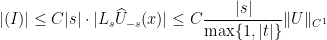
On the other hand, this pointwise bound is not adequate to control 


Lemma 8 There exists a constant
;
,
for all
Proof: Recall that 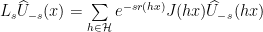
It follows from Lemma 6 that

where 


Let us now prove the second item of the lemma. For this sake, we write 


The fourth term is bounded by
Similarly, the bounded distortion property 

Finally, since 

and the first term is bounded by
(thanks to the estimate from the first item.)
This completes the proof of the lemma.
Remark 9 An important point in this lemma is that the
norm of
.This suggests that we should measure
in order to get some uniform control on the operator
and this is exactly the statement of Lemma 7.18 in AGY paper. This norm will show up again in the statement of the Dolgopyat-like estimate.


Once we have Corollary 7 and Lemma 8, we are ready use the estimate (6) and some classical properties (namely, Lasota-Yorke inequality and weak mixing for
Lemma 9 For any
(of radius independent of
Proof: It is well-known (cf. Lemma 7.8 in AGY paper) that the weighted transfer operator 
By Hennion’s theorem (cf. Baladi’s book), a Lasota-Yorke inequality for 


In other words, if one can show that 


for some constants 


defines an analytic extension to
In summary, we have reduced the proof of the lemma to the verification of the fact that 


This proves the lemma.
Remark 10 A more direct proof of this lemma (without relying on the weak-mixing property for
Next, let us adapt the argument above to perform the step (b) of the Paley-Wiener strategy:
Lemma 10 There exists an open disk
(of radius independent of
Proof: The transfer operator 


Nevertheless, we can overcome this difficulty as follows. For 
where 


In other terms, after we remove from 
At this point, the basic idea is to “repeat” the argument of the proof of Lemma 9 with
(Here, we used that 

Observe that the series 

It follows that we can use the previous equation to define an analytic extension of 

Note that this is a completely obvious task for 
has a pole at
Fortunately, the order of pole at 

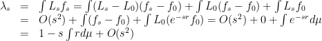
where 


Thus, the function (8) is analytic on 

has a zero at 


and our assumption (2) was precisely that 
This proves the lemma.
Closing this post, let us reduce the step (c) to the following Dolgopyat-like estimate (compare with Proposition 7.7 in AGY paper):
Proposition 11 There exist
,
,
and
for all
,
,
. (Here,
is the norm introduced in Remark 9.)
The proof of this proposition will occupy the next post of this series. For now, let us implement the step (c) of the Paley-Wiener strategy assuming Proposition 11.
We want to use the formula (4) to define a suitable analytic extension

of 
By (6), Proposition 11, Corollary 7 and Lemma 8, we have

for all
This proves that 


Leave a comment