Computation of the Poisson boundary of a lattice of SL(2,R)

Posted by: matheuscmss | August 9, 2013

Computation of the Poisson boundary of a lattice of SL(2,R)

In this previous post, we discussed some results of Furstenberg on the Poisson boundaries of lattices of ${SL(n,\mathbb{R})}$ (mostly in the typical low-dimensional cases ${n=2}$ and/or ${n=3}$ ). In particular, we saw that it is important to know the Poisson boundary of such lattices in order to be able to distinguish between them.

More precisely, using the notations of this post (as well as of its companion), we mentioned that a lattice ${\Gamma}$ of ${SL(n,\mathbb{R})}$ can be equipped with a probability measure ${\mu}$ such that the Poisson boundary of ${(\Gamma,\mu)}$ coincides with the Poisson boundary ${(B_n, m_{B_n})}$ of ${SL(n,\mathbb{R})}$ equipped with any spherical measure (cf. Theorem 13 of this post). Then, we sketched the construction of the probability measure ${\mu}$ in the case of a cocompact lattice ${\Gamma}$ of ${SL(2,\mathbb{R})}$ , and, after that, we outlined the proof that ${(B_n, m_{B_n})}$ is a boundary of ${(\Gamma,\mu)}$ in the cases ${n=2}$ and ${3}$ .

However, we skipped a proof of the fact that ${(B_n, m_{B_n})}$ is the Poisson boundary of ${(\Gamma, \mu)}$ by postponing it possibly to another post. Today our plan is to come back to this point by showing that ${(B_2, m_{B_2})}$ is the Poisson boundary of ${(\Gamma,\mu)}$ .

More concretely, we will show the following statement due to Furstenberg. Let ${\Gamma}$ be a cocompact lattice of ${SL(2,\mathbb{R})}$ . As we saw in this previous post (cf. Proposition 14), one can construct a probability measure ${\mu}$ on ${\Gamma}$ such that

(a) ${\mu}$ has full support: ${\mu(\{\gamma\})>0}$ for all ${\gamma\in\Gamma}$ ,
(b) ${m_{B_2}}$ is ${\mu}$ –stationary: ${\mu\ast m_{B_2}=m_{B_2}}$ ,
(c) the ${\log}$ –norm function is ${\mu}$ –integrable: ${\sum\limits_{\gamma\in\Gamma} \mu(\gamma)\Lambda(\gamma)<\infty}$ .

Here, we recall (for the sake of convenience of the reader) that: ${B_2\simeq\mathbb{P}^1}$ is the “complete flag variety” of ${\mathbb{R}^2}$ or, equivalently, ${B_2=SL(2,\mathbb{R})/P_2}$ where ${P_2}$ is the subgroup of upper-triangular matrices, ${m_{B_2}}$ is the Lebesgue (probability) measure and

$\displaystyle \Lambda(g):=d(g(0),0)=\log\frac{1+|g(0)|}{1-|g(0)|}$

where ${g\in SL(2,\mathbb{R})}$ acts on Poincaré’s disk ${\mathbb{D}}$ via Möebius transformations (as usual) and ${d}$ denotes the hyperbolic distance on Poincaré’s disk ${\mathbb{D}}$ .

Then, the result of Furstenberg that we want to show today is:

Theorem 1 Let ${\Gamma}$ be a cocompact lattice of ${SL(2,\mathbb{R})}$ and denote by ${\mu}$ any probability measure on ${\Gamma}$ satisfying the conditions in items (a), (b) and (c) above. Then, the Poisson boundary of ${(\Gamma,\mu)}$ is ${(B_2, m_{B_2})}$ .

The proof of this theorem will occupy the entire post, and, in what follows, we will assume familiarity with the contents of these posts.

1. Preliminaries

As we already mentioned above, we know that ${(B_2, m_{B_2})}$ is a boundary of ${(\Gamma, \mu)}$ (cf. Subsection 2.2 of this post).

Thus, if we denote by ${(B,\theta)}$ the Poisson boundary of ${(\Gamma, \mu)}$ (an object constructed in Section 4 of this post), then, by the maximality of the Poisson boundary, ${(B_2, m_{B_2})}$ is an equivariant image of ${(B, \theta)}$ under some equivariant map ${\rho: B\rightarrow B_2}$ .

Our goal consists into showing that ${\rho}$ is an isomorphism, and, for this sake, it suffices to show that we can recover all bounded measurable functions of ${(B,\theta)}$ from the corresponding functions on ${(B_2, m_{B_2})}$ via ${\rho}$ , i.e., the proof of Theorem 1 is reduced to prove that:

Proposition 2 All functions ${\widetilde{\phi}\in L^{\infty}(B,\theta)}$ have the form ${\widetilde{\phi}=\phi\circ\rho}$ with ${\phi\in L^{\infty}(B_2,m_{B_2})}$ .

In this direction, it is technically helpful to replace ${L^{\infty}(B,\theta)}$ by ${L^2(B,\theta)}$ and consider the subspace

$\displaystyle V=\{\widetilde{\psi}\in L^2(B,\theta): \widetilde{\psi}=\psi\circ\rho, \, \psi\in L^2(B_2, m_{B_2})\}.$

In fact, since ${V}$ is a closed subspace of the Hilbert space ${L^2(B,\theta)}$ , we have an orthogonal projection ${\pi_V: L^2(B,\theta)\rightarrow V}$ and our task of proving Proposition 2 is equivalent to show that ${\pi_V}$ is the identity map ${\textrm{id}}$ .

Now, the basic strategy to show that ${\pi_V=\textrm{id}}$ is to prove that, for each ${\phi\in L^{\infty}(B,\theta)}$ , the functions ${\phi}$ and ${\pi_V(\phi)}$ induce the same ${\mu}$ -harmonic function on ${\Gamma}$ (via Poisson formula). Indeed, since ${(B,\theta)}$ is the Poisson boundary of ${(\Gamma,\mu)}$ , we have (by definition) that the Poisson formula associates an unique ${\mu}$ -harmonic function

$\displaystyle h_{\phi}(\gamma)=\int_B \phi(\xi)d\gamma\theta(\xi)$

on ${\Gamma}$ to each ${\phi\in L^{\infty}(B,\theta)}$ . Hence, if ${\phi}$ and ${\pi_V(\phi)}$ are associated to the same ${\mu}$ -harmonic function on ${\Gamma}$ , then ${\pi_V(\phi)=\phi}$ . In other words, we reduced the proof of Proposition 2 to the following statement:

Proposition 3 Given ${\phi\in L^{\infty}(B,\theta)}$ , the functions ${\phi}$ and ${\pi_V(\phi)}$ induce the same ${\mu}$ -harmonic function on ${\Gamma}$ via Poisson formula.

In other to show this proposition, we rewrite the ${\mu}$ -harmonic function ${h_{\varphi}}$ associated to ${\phi}$ in terms of the ${L^2}$ -inner product ${\langle .,. \rangle}$ as follows:

$\displaystyle h_{\varphi}(\gamma)=\int_B \varphi(\xi)d\gamma\theta(\xi)=\int_B \varphi(\xi)\frac{d\gamma\theta}{d\theta}(\xi)d\theta(\xi)=\langle\varphi, \frac{d\gamma\theta}{d\theta}\rangle$

In particular, if ${\frac{d\gamma\theta}{d\theta}\in V}$ for all ${\gamma\in \Gamma}$ , then

$\displaystyle h_{\pi_V(\phi)}(\gamma)=\langle\pi_V(\phi),\frac{d\gamma\theta}{d\theta}\rangle = \langle\phi,\pi_V\left(\frac{d\gamma\theta}{d\theta}\right)\rangle=\langle\phi,\frac{d\gamma\theta}{d\theta}\rangle = h_{\phi}(\gamma).$

Equivalently, we just showed that ${\phi}$ and ${\pi_V(\phi)}$ induce the same ${\mu}$ -harmonic function if ${d(\gamma\theta)/d\theta\in V}$ for all ${\gamma\in\Gamma}$ , that is, the proof of Proposition 3 will be complete once we prove that:

Proposition 4 For each ${\gamma\in\Gamma}$ , the function ${d(\gamma\theta)/d\theta}$ belongs to ${V}$ .

As it turns out, the functions ${f\in V}$ admit a nice characterization in terms of Jensen’s inequality. More concretely, since ${V}$ consists of all functions in ${L^2(B,\theta)}$ which are measurable with respect to the field of sets ${\rho^{-1}(A)}$ (with ${A\subset B_2}$ measurable), one can show that the projection ${\pi_V}$ enjoys a “Jensen’s inequality property”:

$\displaystyle \pi_V(\log f)\leq\log\pi_V(f) \ \ \ \ \ (1)$

with equality holding only for functions ${f\in V}$ .

As the reader might suspect, we intend to use Jensen’s inequality to produce an equality characterizing whether ${d(\gamma\theta)/d\theta\in V}$ . For this, we will compute ${\pi_V(f)}$ for ${f=d(\gamma\theta)/d\theta}$ .

In fact, it is not hard to guess who ${\pi_V(d(\gamma\theta)/d\theta)}$ must be: since ${\rho}$ is an equivariant map sending ${\theta}$ to ${m_{B_2}}$ , it is not surprising that ${\pi_V(d(\gamma\theta)/d\theta) = (d(\gamma m_{B_2})/dm_{B_2})\circ\rho}$ . Now, let us formalize this naive guess as follows. Recall that, by definition, ${\pi_V(f)}$ is the (unique) function in ${V}$ such that

$\displaystyle \langle\widetilde{\psi}, \pi_V(f)\rangle = \langle\widetilde{\psi}, f\rangle$

for each ${\widetilde{\psi}\in V}$ , i.e., ${\widetilde{\psi}=\psi\circ\rho}$ with ${\psi\in L^2(B_2,m_{B_2})}$ ). We rewrite this identity as

$\displaystyle \int_B \psi(\rho(\eta))\pi_V(f)(\eta)d\theta(\eta) = \int_B\psi(\rho(\eta))f(\eta)d\theta(\eta).$

For ${f=d(\gamma\theta)/d\theta}$ , this identity becomes

$\displaystyle \int_B \psi(\rho(\eta))\pi_V\left(\frac{d(\gamma\theta)}{d\theta}\right)(\eta)d\theta(\eta) = \int_B\psi(\rho(\eta))\frac{d(\gamma\theta)}{d\theta}(\eta)d\theta(\eta) = \int_B\psi(\rho(\eta))d\gamma\theta(\eta).$

Observe that the right-hand side of this equality is the ${\mu}$ -harmonic function of ${\gamma\in\Gamma}$ induced by ${\psi(\rho(\eta))\in L^{\infty}(B,\theta)}$ . On the other hand, since ${\rho}$ is an equivariant map between the Poisson boundary ${(B,\theta)}$ and the boundary ${(B_2,m_{B_2})}$ , we have that the functions ${\psi(\rho(\eta))\in L^{\infty}(B,\theta)}$ and ${\psi(\xi)\in L^{\infty}(B_2,m_{B_2})}$ induce the same ${\mu}$ -harmonic function, i.e.,

$\displaystyle \int_B\psi(\rho(\eta))d\gamma\theta(\eta)=\int_{B_2}\psi(\xi) d\gamma m_{B_2}(\xi)$

By putting the previous two equalities together, we get that

$\displaystyle \int_B \psi(\rho(\eta))\pi_V\left(\frac{d(\gamma\theta)}{d\theta}\right)(\eta)d\theta(\eta) = \int_{B_2}\psi(\xi) d\gamma m_{B_2}(\xi) = \int_{B_2}\psi(\xi) \frac{d\gamma m_{B_2}}{dm_{B_2}}(\xi)dm_{B_2}(\xi)$

Next, we recall that ${\rho}$ sends ${\theta}$ to ${m_{B_2}}$ (i.e., ${\rho\theta=m_{B_2}}$ ). Therefore, if we denote ${\xi=\rho(\eta)}$ , we obtain that the right-hand side of the previous equality becomes

$\displaystyle \int_{B_2}\psi(\xi) \frac{d\gamma m_{B_2}}{dm_{B_2}}(\xi)dm_{B_2}(\xi)=\int_{B_2}\psi(\xi) \frac{d\gamma m_{B_2}}{dm_{B_2}}(\xi)d\rho\theta(\xi) = \int_{B}\psi(\rho(\eta)) \frac{d\gamma m_{B_2}}{dm_{B_2}}(\rho(\eta))d\theta(\eta)$

By combining the last two equalities above, we deduce that

$\displaystyle \int_B \psi(\rho(\eta))\pi_V\left(\frac{d(\gamma\theta)}{d\theta}\right)(\eta)d\theta(\eta) = \int_{B}\psi(\rho(\eta)) \frac{d\gamma m_{B_2}}{dm_{B_2}}(\rho(\eta))d\theta(\eta).$

Since this identity holds for an arbitrary function ${\psi}$ , we conclude that

$\displaystyle \pi_V\left(\frac{d(\gamma\theta)}{d\theta}\right)(\eta)=\frac{d\gamma m_{B_2}}{dm_{B_2}}(\rho(\eta)),$

as it was claimed (or rather guessed).

From this computation and Jensen’s inequality (1), we get the following lemma:

Lemma 5 For each ${\gamma\in\Gamma}$ one has

$\displaystyle \int_B \log\frac{d\gamma\theta}{d\theta}(\eta)d\theta(\eta)\leq \int_{B_2} \log\frac{d\gamma m_{B_2}}{dm_{B_2}}(\xi)dm_{B_2}(\xi) \ \ \ \ \ (2)$

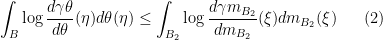
with equality only if the function ${d(\gamma\theta)/d\theta}$ belongs to ${V}$ .

Proof: By setting ${f=d(\gamma\theta)/d\theta}$ , we see that the left-hand side of (2) is

$\displaystyle \langle \log f, 1\rangle=\langle \log f, \pi_V(1)\rangle = \langle \pi_V(\log f), 1\rangle$

while our computation of ${\pi_V(f) (=\pi_V(d(\gamma\theta)/d\theta)=d(\gamma m_{B_2})/dm_{B_2})}$ above reveals that the right-hand side of (2) is

$\displaystyle \langle \log(\pi_V(f)), 1\rangle$

It follows that the desired lemma is a consequence of Jensen’s inequality (1). $\Box$

This lemma reduces to proof of Proposition 4 to show that one has an equality in (2) (for all ${\gamma\in\Gamma}$ ). Here, we claim that it is sufficient to check that

$\displaystyle \sum\limits_{\gamma\in\Gamma} \mu(\gamma)\int_B\log\left(\frac{d\gamma^{-1}\theta}{d\theta}\right)^{-1}d\theta\leq \sum\limits_{\gamma\in\Gamma} \mu(\gamma)\int_{B_2}\log\left(\frac{d\gamma^{-1}m_{B_2}}{dm_{B_2}}\right)^{-1}dm_{B_2} \ \ \ \ \ (3)$

for all ${\gamma\in\Gamma}$ . Indeed, since ${\mu}$ has full support, i.e., ${\mu(\gamma)>0}$ for all ${\gamma\in\Gamma}$ (cf. item (a) above), it follows from (2) and (3) that one has equality in (2) for all ${\gamma\in\Gamma}$ .

In summary, our task now becomes to prove that:

Proposition 6 For all ${\gamma\in\Gamma}$ , the inequality (3) above holds, i.e.,

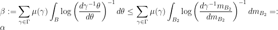
$\displaystyle \beta:=\sum\limits_{\gamma\in\Gamma} \mu(\gamma)\int_B\log\left(\frac{d\gamma^{-1}\theta}{d\theta}\right)^{-1}d\theta\leq \sum\limits_{\gamma\in\Gamma} \mu(\gamma)\int_{B_2}\log\left(\frac{d\gamma^{-1}m_{B_2}}{dm_{B_2}}\right)^{-1}dm_{B_2}=:\alpha$

The basic idea to prove this proposition is the following. The quantities ${\alpha}$ and ${\beta}$ can be interpreted as spatial averages. In particular, the ergodic theorem will tell us that ${\alpha}$ and ${\beta}$ drive the Birkhoff sums of the observables ${d\gamma^{-1}m_{B_2}/dm_{B_2}}$ and ${d\gamma^{-1}\theta/d\theta}$ along almost every sample of random walk in ${\Gamma}$ .

Now, assuming by contradiction that ${\beta>\alpha}$ , we will see that the Birkhoff sums of ${d\gamma^{-1}\theta/d\theta}$ are very well controlled by the Birkhoff sums of ${d\gamma^{-1}m_{B_2}/dm_{B_2}}$ (with some “margin” coming from the strict inequality ${\beta>\alpha}$ ). Using this and the fact that the density ${d\gamma^{-1}m_{B_2}/dm_{B_2}}$ can be explicitly computed, we will be able to solve a counting problem to show that:

Proposition 7 If ${\beta>\alpha}$ , then there exists a recurrence subset ${\Delta}$ of ${\Gamma}$ (i.e., a subset that is hit by the random walk infinitely often with probability ${1}$ ) with the property that

$\displaystyle \sum\limits_{\gamma\in\Delta}\left\|\frac{d\gamma\theta}{d\theta}\right\|_{L^{\infty}}^{-1}<\infty$

On the other hand, using the properties of ${\mu}$ -harmonic functions, we will show the following general fact about recurrence sets of ${\Gamma}$ :

Proposition 8 Let ${\Delta}$ be a recurrence set of ${\Gamma}$ for the random walk ${y_1\dots y_n}$ associated to a stationary sequence ${\{y_n\}}$ of independent random variables with distribution ${\mu}$ . Then,

$\displaystyle \sum\limits_{\gamma\in\Delta}\left\|\frac{d\gamma\theta}{d\theta}\right\|_{L^{\infty}}^{-1}=\infty$

Of course, by putting together Propositions 7 and 8, we deduce the validity of Proposition 6. Hence, it remains only to prove Propositions 7 and 8. In order to organize the discussion, we will show them in separate sections, namely, the next section will concern Proposition 7 while the final section of this post will concern Proposition 8.

2. Proof of Proposition 7

As we already mentioned above, the first step in the proof of this proposition is to observe that ${\alpha}$ and ${\beta}$ are spatial averages, so that the ergodic theorem says that one can express them in terms of temporal averages along typical “orbits” (samples of random walk).

More precisely, let ${\{y_n\}}$ be a stationary sequence of independent random variables with distribution ${\mu}$ and consider ${\{z_n\}}$ the ${\mu}$ -process on ${B}$ . For technical reasons (that will become clear in a moment), we will think of ${\{z_n\}}$ as moving forward in time (rather than backward), i.e., the ${\mu}$ -process ${\{z_n\}}$ satisfies

$\displaystyle z_{n+1} = y_{n+1} z_n$

with ${y_{n+1}}$ independent of ${z_n, z_{n-1},\dots}$ (instead of ${z_n=y_n z_{n+1}}$ and ${y_n}$ independent of ${z_{n+1}, z_{n+2},\dots}$ ). Note that by setting

$\displaystyle w_n=\rho(z_n)$

we get a ${\mu}$ -process on ${B_2}$ (because ${\rho}$ is an equivariant map from ${(B,\theta)}$ to ${(B_2,m_{B_2})}$ ).

2.1. Interpretation of ${\alpha}$ as a Birkhoff sum

In this language, we can convert the spatial average ${\alpha}$ of the observable

$\displaystyle \log\left(\frac{d\gamma^{-1}m_{B_2}}{dm_{B_2}}\right)^{-1}$

in a Birkhoff average as follows. Let us consider the random walk ${\gamma=y_n\dots y_1}$ on ${\Gamma}$ obtained by left-multiplication. Then,

$\displaystyle \begin{array}{rcl} & &\log\left(\frac{d(y_n\dots y_1)^{-1}m_{B_2}}{dm_{B_2}}(w_0)\right)^{-1} = \sum\limits_{i=0}^{n-1} \log\left(\frac{d(y_1^{-1}\dots y_{i+1}^{-1})m_{B_2}}{d(y_1^{-1}\dots y_{i}^{-1})m_{B_2}}(w_0)\right)^{-1} \\ &=& \sum\limits_{i=0}^{n-1} \log\left(\frac{dy_{i+1}^{-1}m_{B_2}}{dm_{B_2}}(y_{i}\dots y_1 w_0)\right)^{-1} = \sum\limits_{i=0}^{n-1} \log\left(\frac{dy_{i+1}^{-1}m_{B_2}}{dm_{B_2}}(w_i)\right)^{-1} \end{array}$

By applying the ergodic theorem to the right-hand side of this expression (and using the fact that ${y_i}$ and ${w_{i-1}}$ are independent), we obtain that

$\displaystyle \log\left(\frac{d(y_n\dots y_1)^{-1}m_{B_2}}{dm_{B_2}}(w_0)\right)^{-1}\sim n\alpha \ \ \ \ \ (4)$

Of course, in order to justify the application of the ergodic theorem, we need to check the (absolute) integrability of the corresponding observable, that is, we need to show that the following expectation

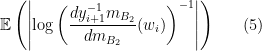
$\displaystyle \mathbb{E}\left(\left|\log\left(\frac{dy_{i+1}^{-1}m_{B_2}}{dm_{B_2}}(w_i)\right)^{-1}\right|\right) \ \ \ \ \ (5)$

is finite.

As it turns out, the finiteness of this expectation is a consequence of the integrability condition on ${\mu}$ in item (c) above. Indeed, we have

$\displaystyle \mathbb{E}\left(\left|\log\left(\frac{dy_{i+1}^{-1}m_{B_2}}{dm_{B_2}}(w_i)\right)^{-1}\right|\right)\leq \mathbb{E}\left(\max\limits_{\xi} \left|\log\left(\frac{dy_{i+1}^{-1}m_{B_2}}{dm_{B_2}}(\xi)\right)^{-1}\right|\right) \ \ \ \ \ (6)$

and, in general, the quantity

$\displaystyle \max\limits_{\xi} \left|\log\left(\frac{dg^{-1}m_{B_2}}{dm_{B_2}}(\xi)\right)^{-1}\right|$

can be controlled as follows. By letting ${g\in SL(2,\mathbb{R})}$ act on the Poincaré’s disk ${\mathbb{D}}$ via

$\displaystyle g(z)=\rho\frac{z+a}{1+\overline{a}z}$

where ${|\rho|=1}$ and ${a\in\mathbb{D}}$ . We have that

$\displaystyle \frac{dg^{-1}m_{B_2}}{dm_{B_2}}(\xi) = |g'(\xi)|=\frac{1-|a|^2}{|1+\overline{a}\xi|^2}=\frac{1-|g(0)|^2}{|1+\overline{a}\xi|^2}$

A simple calculation using this expression and the fact that ${\Lambda(g):=\log\frac{1+|g(0)|}{1-|g(0)|}}$ reveals that

$\displaystyle \max\limits_{\xi} \left|\log\left(\frac{dg^{-1}m_{B_2}}{dm_{B_2}}(\xi)\right)^{-1}\right|\leq\log 4 + \Lambda(g)$

Therefore, from the ${\mu}$ -integrability of ${\Lambda}$ , cf. item (c) above, we deduce that

$\displaystyle \mathbb{E}\left(\max\limits_{\xi} \left|\log\left(\frac{dy_{i+1}^{-1}m_{B_2}}{dm_{B_2}}(\xi)\right)^{-1}\right|\right)<\infty$

and, in view of (6), we conclude the integrability of (5).

In summary, the validity of (4) essentially follows from the ${\mu}$ -integrability condition on ${\Lambda}$ in item (c).

2.2. Interpretation of ${\beta}$ as a Birkhoff sum

Similarly to the case of ${\alpha}$ , we want to convert ${\beta}$ into Birkhoff average. Again, let us consider the random walk ${\gamma=y_n\dots y_1}$ on ${\Gamma}$ , and let us write

$\displaystyle \begin{array}{rcl} & &\log\left(\frac{d(y_n\dots y_1)^{-1}\theta}{d\theta}(z_0)\right)^{-1} = \sum\limits_{i=0}^{n-1} \log\left(\frac{d(y_1^{-1}\dots y_{i+1}^{-1})\theta}{d(y_1^{-1}\dots y_{i}^{-1})\theta}(z_0)\right)^{-1} \\ &=& \sum\limits_{i=0}^{n-1} \log\left(\frac{dy_{i+1}^{-1}\theta}{d\theta}(y_{i}\dots y_1 z_0)\right)^{-1} = \sum\limits_{i=0}^{n-1} \log\left(\frac{dy_{i+1}^{-1}\theta}{d\theta}(z_i)\right)^{-1} \end{array}$

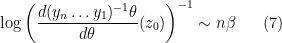
We want to apply once more the ergodic theorem to obtain

$\displaystyle \log\left(\frac{d(y_n\dots y_1)^{-1}\theta}{d\theta}(z_0)\right)^{-1}\sim n\beta \ \ \ \ \ (7)$

However, the justification of the application of the ergodic theorem is a little bit more subtle because the (absolute) integrability of

$\displaystyle \mathbb{E}\left(\left|\log\left(\frac{dy_{i+1}^{-1}\theta}{d\theta}(z_i)\right)^{-1}\right|\right) \ \ \ \ \ (8)$

might be not true. Indeed, we have no prior information on the relationship between ${dg^{-1}\theta/d\theta}$ and ${\Lambda(g)}$ , so that we can not use item (c) to get the integrability (contrary to the case of the Lebesgue measure ${m_{B_2}}$ where ${dg^{-1}m_{B_2}/dm_{B_2}}$ could be computed explicitly). Fortunately, it is not hard to overcome this little technical difficulty: as it turns out, the ergodic theorem also applies to observables that are bounded only on one side by a ${\mu\times\theta}$ -integrable function; in particular, we can apply the ergodic theorem to ${-\log d\gamma^{-1}\theta/d\theta}$ because

$\displaystyle \int\log^+\left(\frac{d\gamma^{-1}\theta}{d\theta}(\eta)\right)d\theta(\eta)\leq\int\frac{d\gamma^{-1}\theta}{d\theta}(\eta)d\theta(\eta)=1$

2.3. Construction of a “weird” recurrence set ${\Delta}$ when ${\beta>\alpha}$

During this subsection, let us assume that ${\beta>\alpha}$ . Recall that the plan is to show that the Birkhoff sums of of ${d\gamma^{-1}\theta/d\theta}$ are very well controlled by the Birkhoff sums of ${d\gamma^{-1}m_{B_2}/dm_{B_2}}$ .

In this direction, let us observe that the asymptotics in (4) and (7) imply

$\displaystyle \lim\limits_{n\rightarrow\infty}\frac{\log\left(\frac{d(y_n\dots y_1)^{-1}\theta}{d\theta}(z_0)\right)^{-1}}{\log\left(\frac{d(y_n\dots y_1)^{-1}m_{B_2}}{dm_{B_2}}(w_0)\right)^{-1}}=\frac{\beta}{\alpha}\leq\infty \ \ \ \ \ (9)$

Using the properties of the Radon-Nikodym derivative (e.g., ${\frac{d\phi m}{d\phi n}(x)=\frac{dm}{dn}(\phi^{-1}(x))}$ ), we can rewrite the numerator in the left-hand side of this equation as:

$\displaystyle \left(\frac{d(y_n\dots y_1)^{-1}\theta}{d\theta}(z_0)\right)^{-1} = \left(\frac{d\theta}{d(y_n\dots y_1)\theta}(y_n\dots y_1 z_0)\right)^{-1} = \frac{d(y_n\dots y_1)\theta}{d\theta}(z_n)$

From this and (9) we deduce that

$\displaystyle \liminf\limits_{n\rightarrow\infty}\frac{\log\left\|\frac{d(y_n\dots y_1)\theta}{d\theta}\right\|_{L^{\infty}}}{\log\left(\frac{d(y_n\dots y_1)^{-1}m_{B_2}}{dm_{B_2}}(w_0)\right)^{-1}}\geq\frac{\beta}{\alpha} \ \ \ \ \ (10)$

with probability ${1}$ . Since ${y_i}$ ‘s are independent of ${w_0}$ , we conclude from (11) that, for almost every ${w_0}$ , one has

for almost all random paths ${\{y_n\}}$ .

In particular, we can fix two distinct values ${\xi_1}$ and ${\xi_2}$ of ${w_0}$ so that (11) holds for almost every random path. For ${i=1, 2}$ , let us consider the random variables

$\displaystyle u_n^{(i)}:=\frac{\log\left\|\frac{d(y_n\dots y_1)\theta}{d\theta}\right\|_{L^{\infty}}}{\log\left(\frac{d(y_n\dots y_1)^{-1}m_{B_2}}{dm_{B_2}}(w_0)\right)^{-1}}$

and

$\displaystyle v_n^{(i)}:=\frac{\log\left\|\frac{d(y_1\dots y_n)\theta}{d\theta}\right\|_{L^{\infty}}}{\log\left(\frac{d(y_1\dots y_n)^{-1}m_{B_2}}{dm_{B_2}}(w_0)\right)^{-1}}$

We are interested in the properties of ${v_n^{(i)}}$ (as ${y_1\dots y_n}$ is the random walk on ${\Gamma}$ ) but (11) provides information only about ${u_n^{(i)}}$ . Fortunately, ${u_n^{(i)}}$ and ${v_n^{(i)}}$ have the same distribution, so that all probabilistic statements about ${u_n^{(i)}}$ are also true for ${v_n^{(i)}}$ . In particular, for each ${\varepsilon>0}$ , the probabilities of the events

$\displaystyle \{v_n^{(i)}<(\beta/\alpha)-\varepsilon\}$

go to ${0}$ for ${i=1, 2}$ because the probabilities of the events

$\displaystyle \{u_n^{(i)}<(\beta/\alpha)-\varepsilon\}$

go to ${0}$ for ${i=1, 2}$ in view of the fact that (11) implies

$\displaystyle \liminf\limits_{n\rightarrow\infty} u_n^{(i)}\geq\beta/\alpha$

with probability ${1}$ (for ${i=1, 2}$ ).

Therefore, if we choose a sequence ${n_k=n_k(\varepsilon)\in\mathbb{N}}$ going very fast to infinity as ${k\rightarrow\infty}$ so that the sum of the probabilities of the events

$\displaystyle \{v_{n_k}^{(i)}<(\beta/\alpha)-\varepsilon\}$

is finite (for ${i=1, 2}$ ), then we can use the Borel-Cantelli lemma to obtain that

$\displaystyle \liminf\limits_{k\rightarrow\infty} v_{n_k}^{(i)}\geq(\beta/\alpha)-\varepsilon$

with probability ${1}$ . In particular, it follows that the set

$\displaystyle \Delta=\left\{\gamma\in\Gamma: \frac{\log\left\|\frac{d\gamma\theta}{d\theta}\right\|_{L^{\infty}}}{\log\left(\frac{d\gamma^{-1}m_{B_2}}{dm_{B_2}}(\xi_i)\right)^{-1}}\geq \frac{\beta}{\alpha}-2\varepsilon \, \textrm{ for } \, i=1, 2\right\}$

is a recurrence set for the random walk ${y_1\dots y_n}$ (i.e., this random walk visits ${\Delta}$ infinitely often with probability ${1}$ ).

Now, if ${\beta>\alpha}$ , we can take ${\varepsilon>0}$ and ${\tau\in\mathbb{R}}$ such that

$\displaystyle 1<\tau<\frac{\beta}{\alpha}-2\varepsilon,$

then any ${\gamma\in\Delta}$ satisfies

$\displaystyle \log\left\|\frac{d\gamma\theta}{d\theta}\right\|_{L^{\infty}}\geq \tau\log\left(\frac{d\gamma^{-1}m_{B_2}}{dm_{B_2}}(\xi_i)\right)^{-1} \textrm{ for } i=1, 2. \ \ \ \ \ (12)$

In other words, the density ${d\gamma\theta/d\theta}$ is very well-controlled by ${\max\limits_{i=1, 2}\frac{d\gamma^{-1}m_{B_2}}{dm_{B_2}}(\xi_i)}$ with a “margin” ${\tau>1}$ coming from the assumption that ${\beta>\alpha}$ .

From this nice control our plan is to prove that the recurrence set ${\Delta}$ has the “weird” property referred to in Proposition 7, i.e., we will show that

$\displaystyle \sum\limits_{\gamma\in\Delta}\left\|\frac{d\gamma\theta}{d\theta}\right\|_{L^{\infty}}^{-1}<\infty.$

Keeping this goal in mind, given ${L>0}$ , let us denote by

$\displaystyle n(L):=\#\left\{\gamma\in\Delta: \left\|\frac{d\gamma\theta}{d\theta}\right\|_{L^{\infty}}<\exp(\tau L)\right\}$

By (12), we can bound the quantity ${n(L)}$ as follows:

$\displaystyle n(L)\leq N(L):=\#\left\{\gamma\in\Delta: \max\limits_{i=1, 2} \left(\frac{d\gamma^{-1}m_{B_2}}{dm_{B_2}}(\xi_i)\right)^{-1} < \exp(L)\right\}$

In particular, if we write

$\displaystyle \sum\limits_{\gamma\in\Delta}\left\|\frac{d\gamma\theta}{d\theta}\right\|_{L^{\infty}}^{-1}=\sum\limits_{L\in\mathbb{N}}\sum\limits_{\gamma\in\Delta_L}\left\|\frac{d\gamma\theta}{d\theta}\right\|_{L^{\infty}}^{-1} \ \ \ \ \ (13)$

where

$\displaystyle \Delta_L:=\left\{\gamma\in\Gamma: \exp(\tau L)<\left\|\frac{d\gamma\theta}{d\theta}\right\|_{L^{\infty}}<\exp(\tau (L+1))\right\}$

and we observe that ${\#\Delta_L\leq n(L+1)\leq N(L+1)}$ , we can estimate the right-hand side of (13) as

Since ${\tau}$ was chosen so that ${\tau>1}$ (assuming ${\beta>\alpha}$ ), we have that the right-hand side of this estimate is convergent if we can show that ${\log N(L)}$ grows linearly (at most), i.e., the proof of Proposition 7 is complete once we can handle the counting problem of showing that

Lemma 9 ${\log N(L)\sim L}$ as ${L\rightarrow\infty}$ .

We will exploit the explicit nature of the densities ${\left(\frac{d\gamma^{-1}m_{B_2}}{dm_{B_2}}(\xi_i)\right)^{-1}}$ in order to show this (counting) lemma. More precisely, given ${g\in SL(2,\mathbb{R})}$ , recall that

$\displaystyle \frac{dg^{-1}m_{B_2}}{dm_{B_2}}(\xi)=|g'(\xi)|=\frac{1-|a|^2}{|1+\overline{a}\xi|^2}=\frac{1-|g(0)|^2}{|1+\overline{a}\xi|^2}$

if ${g}$ acts on Poincaré’s disk ${\mathbb{D}}$ as ${g(z)=\rho(z+a)/(1+\overline{a}z)}$ with ${|\rho|=1}$ and ${a\in\mathbb{D}}$ .

Since ${\xi_1}$ and ${\xi_2}$ are distinct, the complex number ${a}$ can’t be close to both of them at the same time. Using this information, the reader can see that

$\displaystyle a_1(1-|g(0)|^2)<\min\{|g'(\xi_1)|, |g'(\xi_2)|\}<a_2(1-|g(0)|^2)$

for some constants ${a_1=a_1(\xi_1, \xi_2)}$ and ${a_2=a_2(\xi_1,\xi_2)}$ . Equivalently, since ${\Lambda(g)=\log\frac{1+|g(0)|}{1-|g(0)|}}$ , one has

$\displaystyle b_1+\Lambda(\gamma)<\max\left\{\left(\frac{d\gamma^{-1}m_{B_2}}{dm_{B_2}}(\xi_i)\right)^{-1} : i=1, 2\right\}<b_2+\Lambda(\gamma)$

for some constants ${b_1=b_1(\xi_1, \xi_2)}$ and ${b_2=b_2(\xi_1,\xi_2)}$ .

In particular, Lemma 9 is equivalent to show that ${\log N_1(L)\sim L}$ where

$\displaystyle N_1(L)=\#\{\gamma\in\Gamma: d(\gamma(0), 0):=\Lambda(\gamma)<L\}.$

Actually, since the subset of elements ${\gamma\in\Gamma}$ with ${\gamma(0)=0}$ is finite (namely, it is the intersection of the lattice ${\Gamma}$ with the compact subgroup ${SO(2,\mathbb{R})}$ stabilizing ${0}$ ), we can convert the counting problem

$\displaystyle \log N_1(L)\sim L$

for elements of ${\gamma\in\Gamma}$ into the following geometrical counting problem about points ${\gamma(0)\in\mathbb{D}}$ :

$\displaystyle \log N_2(L)\sim L$

where

$\displaystyle N_2(L):=\#\{\gamma(0)\in\mathbb{D}: \gamma\in\Gamma, \, d(\gamma(0), 0)<L\}$

Now, this geometrical counting problem is not hard to solve, at least when ${\Gamma}$ is cocompact.

Indeed, let us consider first ${Q^{(\infty)}}$ a large compact subset of ${\mathbb{D}}$ containing a fundamental domain of ${\Gamma}$ about the origin ${0\in\mathbb{D}}$ . Then, by definition, the ${\Gamma}$ -translates of ${Q^{(\infty)}}$ cover ${\mathbb{D}}$ and, hence,

$\displaystyle N_2(L)>c_1 A(L)$

where ${c_1}$ is an appropriate constant (depending on ${Q^{(\infty)}}$ ) and ${A(L)}$ is the area of the hyperbolic disk of radius ${L}$ centered at ${0}$ .

Next, let us consider ${Q^{(0)}}$ a small compact ball of ${\mathbb{D}}$ around ${0}$ so that it is disjoint from its ${\Gamma}$ -translates. Then, we have that

$\displaystyle N_2(L)<c_2 A(L+1)$

where ${c_2}$ is an appropriate constant (depending on ${Q^{(0)}}$ ).

In summary, there are two constants ${c_1}$ and ${c_2}$ such that

$\displaystyle c_1 A(L)< N_2(L)<c_2 A(L+1)$

On the other hand, the area ${A(L)}$ of the hyperbolic disk ${B_L(0)}$ of radius ${L}$ centered at ${0}$ is not hard to compute:

$\displaystyle A(L)=\int_0^{2\pi}\int_0^{r(L)} \frac{r dr d\theta}{(1-r^2)^2}=2\pi\left(\frac{1}{1-r_L^2}-1\right)$

where ${r_L}$ is the Euclidean radius of ${B_L(0)}$ , i.e., ${L=\log\frac{1+r_L}{1-r_L}}$ . From this expression we see that

$\displaystyle \log A(L)\sim L,$

so that this ends the proof of Lemma 9.

This completes the proof of Proposition 7.

3. Proof of Proposition 8

Closing this post, let us show that the properties of ${\mu}$ -harmonic functions do not allow the existence of the “weird” recurrence sets constructed in Proposition 7. For this sake, let us suppose by contradiction that ${\Delta}$ is a recurrence subset of ${\Gamma}$ such that

$\displaystyle \sum\limits_{\gamma\in\Delta} \left\|\frac{d\gamma\theta}{d\theta}\right\|_{L^{\infty}}^{-1}<\infty$

By removing finitely many elements of ${\Delta}$ if necessary, we get a recurrence set that we still denote ${\Delta}$ such that

$\displaystyle \sum\limits_{\gamma\in\Delta} \left\|\frac{d\gamma\theta}{d\theta}\right\|_{L^{\infty}}^{-1}<1 \ \ \ \ \ (14)$

Next, let us observe the following facts. Firstly, since ${\theta}$ is ${\mu}$ -stationary and ${\mu}$ is fully supported on ${\Gamma}$ (cf. item (a) above), we have that ${\gamma\theta}$ is absolutely continuous with respect to ${\theta}$ and the density ${d\gamma\theta/d\theta}$ is bounded because

$\displaystyle \theta=\mu\ast\theta=\sum\limits_{\gamma\in\Gamma}\mu(\gamma)\gamma\theta$

so that ${\gamma\theta\leq (1/\mu(\gamma))\theta}$ . Secondly, from the previous identity, we see that

$\displaystyle \frac{d\gamma\theta}{d\theta}(\xi) = \sum\limits_{\eta\in\Gamma} \mu(\eta)\frac{d\gamma\eta\theta}{d\theta}(\xi),$

so that, for almost every ${\xi}$ , the function

$\displaystyle \gamma\mapsto\frac{d\gamma\theta}{d\theta}(\xi)$

is ${\mu}$ -harmonic.

In particular, our plan is to use the mean value property of ${\mu}$ -harmonic functions to express the values of ${d\gamma\theta/d\theta}$ in terms of its values in ${\Delta}$ in order to eventually contradict (14).

For this sake, let us show the following elementary abstract lemma about the mean value property of bounded ${\mu}$ -harmonic functions with respect to recurrence sets:

Lemma 10 Let ${G}$ be a discrete group with a probability measure ${\mu}$ and denote by ${\{x_n\}}$ a stationary sequence of independent random variables with distribution ${\mu}$ . If ${R}$ is a recurrence set of the random walk ${x_1\dots x_n}$ and ${h(g)}$ is a bounded ${\mu}$ -harmonic function on ${G}$ , then the following mean value property with respect to ${R}$ holds:

$\displaystyle h(g)=\sum\limits_{g^*\in R}\theta_g(g^*) h(g^*)$

where ${\theta_g}$ is the distribution of the first point of ${R}$ hit by ${gx_1\dots x_n}$ .

Proof: We start with the usual mean value property

$\displaystyle h(g)=\sum\limits_{g'\in G} \mu(g')h(gg')$

Now, for each term ${h(gg')}$ we can independently decide whether we want to use again the mean value relation to express ${h(gg')}$ as a convex combination of ${h(gg'g'')}$ or not. Since our ultimate goal is to write ${h(g)}$ as a convex combination of the values of ${h}$ on the recurrence set ${R}$ , we will take our decision as follows: if ${gg'\in R}$ , we leave ${h(gg')}$ alone, and, otherwise, we apply the mean value relation.

After ${n}$ steps of this procedure, we have

$\displaystyle h(g) = \sum\limits_{g^*\in R}\theta_g^{(n)}(g^*) h(g^*) + \textrm{``something''}$

where “something” is a combined weight of contributions coming from the values of ${h}$ on points outside ${R}$ that were reached by the random walk after ${n}$ steps.

Because ${R}$ is a recurrence set, the random walk reaches ${R}$ with probability ${1}$ . Therefore, since the function ${h}$ is bounded, we can pass to the limit as ${n\rightarrow\infty}$ in the identity above to get the desired equality

$\displaystyle h(g)=\sum\limits_{g^*\in R}\theta_g(g^*) h(g^*)$

This proves the lemma. $\Box$

Coming back to the context of Proposition 8, we observe that this lemma does not apply directly to the ${\mu}$ -harmonic density function

$\displaystyle \frac{d\gamma\theta}{d\theta}(\xi)$

because it might be unbounded.

Nevertheless, by revisiting the argument of the proof of the lemma above, one can easily check that, for an unbounded ${\mu}$ -harmonic (integrable) function ${h}$ , one has the mean value inequality

$\displaystyle h(e)\geq \sum\limits_{\gamma\in\Gamma} p(\gamma) h(\gamma)$

(but possibly not the mean value equality ${h(e)=\sum\limits_{\gamma\in\Gamma} p(\gamma) h(\gamma)}$ ) where ${p(\gamma)}$ is the probability that the first point of ${\Delta}$ hit by the random walk is ${\gamma}$ .

In any event, using this mean value inequality with ${h(g)=\frac{dg\theta}{d\theta}(\xi)}$ we deduce that

$\displaystyle 1\geq \sum\limits_{\gamma\in\Delta} p(\gamma) \frac{d\gamma\theta}{d\theta}(\xi)$

for almost every ${\xi}$ .

In particular, we conclude that

$\displaystyle p(\gamma)\left\|\frac{d\gamma\theta}{d\theta}\right\|_{L^{\infty}}\leq 1.$

Thus, in view of (14), we obtain that

$\displaystyle \sum\limits_{\gamma\in\Delta} p(\gamma)<1,$

that is, the total probability that the random walk hits ${\Delta}$ is strictly smaller than ${1}$ , a contradiction with the fact that ${\Delta}$ is a recurrence set of the random walk!

This completes the proof of Proposition 8, and, hence, this finishes the sketch of proof of Furstenberg’s Theorem 1.

Posted in expository, math.DS, Mathematics | Tags: examples of Poisson boundaries, Hillel Furstenberg, Poisson boundary

M	T	W	T	F	S	S
			1	2	3	4
5	6	7	8	9	10	11
12	13	14	15	16	17	18
19	20	21	22	23	24	25
26	27	28	29	30	31

	Adam on Breuillard-Sert’s joint…
	Adam on Breuillard-Sert’s joint…
	Writing a Hilbert C*… on ERT16: Compact extensions
	matheuscmss on Yoccoz book collection at…
	Jairo B. on Yoccoz book collection at…

Disquisitiones Mathematicae