The concept of mass in General Relativity and its applications

Hi! Today I’m posting an expanded version of an informal talk (directed to PhD students at IMPA) I gave in January 21, 2005 about the so-called ADM mass in General Relativity and its applications. The spirit of the talk was strongly inspired by the famous article “The unreasonable effectiveness of Mathematics in the Natural Sciences” of the Nobel laureate Eugene Wigner. In fact, my goal was to present a beautiful chapter of the interaction between Differential Geometry (Mathematics) and General Relativity (Physics).

–Introduction–

The “unreasonably effective” relationship between Mathematics and Physics is widely known: for instance, it was the lack of an adequate language to understand the so-called Classical Mechanics (Physics) lead Isaac Newton and Gottfried Leibniz (independently) to the foundations of Differential and Integral Calculus.

The bulk of the current discussion is the non-technical presentation of the beautiful interaction between Mathematics and Physics appearing in the definition of the ADM mass in General Relativity and its application (by Richard Schoen) to the solution of the Yamabe problem in Differential Geometry. More precisely, our general plan is the following:

• in the next section, we’ll see how Mathematics helped Physics with the rigorous description of a global definition of mass in General Relativity; in order to do so, we’ll briefly review some of the history of Newtonian Mechanics, Maxwell’s theory of Electromagnetism and Einstein’s (Special and General) theory of Relativity; after that, we’ll introduce Schwarzschild solution to Einstein’s equation (modelling a black hole) and the concept of ADM mass (named after the three physicists Arnowitt, Deser and Misner); finally, we’ll illustrate the effectiveness of Mathematical tools in Physics with some comments about R. Schoen and S.T. Yau proof of the positivity of the ADM mass (via some arguments from the geometry of minimal surfaces);
• in the last section, we’ll illustrate the effectiveness of Physical tools in Mathematics with a rough sketch of R. Schoen solution to the Yamabe problem (via the positivity of the ADM mass).

Before closing the introduction, let me say that this particularly beautiful interaction between Differential Geometry and General Relativity certainly motivates the following extension of the title of Wigner’s article:

“The unreasonable effectiveness of Mathematics in the Natural Sciences and vice-versa“

Also I would like to acknowledge my friend Fernando Coda Marques who patiently explained me the ideas and technical details appearing in R. Schoen’s solution to Yamabe problem and its relationship with the ADM mass in General Relativity. Of course, this talk is an outcome of our discussions (although the mistakes and errors below are my sole responsibility, of course).

–Mathematics helping Physics–

Newtonian Mechanics. In 1642, Sir Isaac Newton proposed a theory (nowadays called Newtonian Mechanics in his honor) whose central goal was the description of the trajectory of a given body via certain Ordinary Differential Equations (ODEs): for instance, given a certain body and denoting by the time variable, its position at time , its velocity at time and its acceleration at time , we have

Furthermore, Newton’s second law allows to understand the trajectory of a body via its mass and the net external force :

In fact, the knowledge of the mass and the force permits to use Newton’s second law to compute the acceleration (and, a posteriori, the velocity and the position ).

Of course, this is a very crude resume of Newton’s theory (which contains several other fundamental principles such as the law of conservation of energy), but one of the basic philosophy is that Newton’s theory gives a precise description about how the presence of an external force interferes with the movement of a given object.

However, even after the consolidation of Newtonian Mechanics, a serious drawback was the fact that this theory was unable to answer the following question:

What is the origin of the forces?

Newton’s law of universal gravitation. In 1687, after important contributions of Galileo Galillei, Isaac Newton answered the previous question with the introduction of Newton’s law of universal gravitation: it says that two objects of masses and at distance are mutually attracted by a force (called gravitational force) whose intensity is

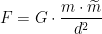
where is a numerical constant (of known value) called gravitational constant.

Again, Isaac Newton obtained a great success because his universal gravitation theory was very accurate (specially concerning its applications to the movement of celestial bodies, such as the Sun, Earth, etc.). However, Newton’s universal gravitation theory left open the following pertinent question:

How the gravitational forces are transmitted?

Before passing to this important question, let us see another (even more serious) problem with the Newtonian Mechanics which became apparent with the advent of Maxwell’s Electromagnetic theory

Maxwell’s Electromagnetism. In 1895, after the advent of new phenomena (namely, electricity and magnetism) without any explanation in Newton’s theory lead the Scottish physicist James C. Maxwell to the development of his Electromagnetic theory. In crude terms, this theory says that electricity and magnetism can be understood as an unique object called electromagnetic wave whose dynamics is described by a set of 4 Partial Differential Equations (known as Maxwell equations). An astonishing consequence of Maxwell equations is the fact that electromagnetic waves (such as light) in the vacuum always travels with constant speed (called speed of light). Evidently, Maxwell theory was a great achievement (due to its accurate description of electromagnetic phenomena), but, after the initial excitement, a serious dilemma between Newton and Maxwell theories emerged, as we are going to see below.

A paradox between Newton and Maxwell. Let’s see what happens when we try to measure the velocity of light of a laser beam using Newton and Maxwell theories. From Newton’s point of view, the speed of light measured by an inertial referential, i.e., a referential moving with constant velocity should be (depending whether the referential moves in an opposite direction or in the same direction of the laser beam). But, from Maxwell’s point of view, the speed of light should be in any inertial referential!

A frustrating aspect of this paradox is the fact that Newton theory is very accurate in Celestial Mechanics and Maxwell theory is very accurate in Electromagnetism. Thus, the solution of this paradox became a basilar problem in Physics. Here, an young brilliant German man working at the patent office in Bern (Swiss) comes to the rescue: of course, I’m talking about Albert Einstein.

Special Relativity of Albert Einstein. In 1905, Albert Einstein solved the paradox between Newton and Maxwell with the introduction of the notion of space-time: the basic idea is that the time and the space can’t be considered as two distinct entities because they are an unique object. In fact, using the point of view of space-time, Einstein postulated that any object moves at the speed of light in space-time! At a first glance, you can imagine that this is a misprint since you’re probably sit down comfortably in your chair reading this post and it is clear that you’re not moving at the speed of light. However, you should read Einstein’s postulate more carefully: he says that we are moving at light speed in space-time. In other words, denoting by your velocity vector in space-time, it has coordinates where are the spatial part of and is the temporal part of and Einstein’s postulate says that

In particular, while you may not be moving in space (i.e., ), the fact that you’re moving with the speed of light in space-time simply means that , i.e., from your point of view the time passes with the speed of light. An immediate (and interesting) consequence of this postulate is the fact that the time slows down when we move fast in space (i.e., decreases if we increase ): a popular way of quoting this consequence is “time is relative” (since the way you feel its passage changes depending on the modulus of your spatial velocity).

Furthermore, Einstein formulated his famous formula

relating mass and energy (this is the analog of in Newtonian Mechanics), etc. In resume, Einstein solved the paradox between Newton and Maxwell via a profound (and highly non-trivial) modification of Newton’s laws. However, the attentive reader noticed that we intentionally skipped one question: although Einstein solved the previous paradox, his Special Relativity theory doesn’t explain how the gravitational forces are transmitted. As we are going to see below, the final answer to this subtle question came only after 10 years of hard work of Einstein.

General Relativity of Albert Einstein. In 1915, Einstein formulated the crucial postulate explaining the transmission of gravitational forces: the presence of mass changes the geometry of the space-time — more precisely, it becomes “curved” around massive objects. A nice pictorial description of this phenomena can be found here. Roughly speaking, the idea is that the space-time is a thin rubber leaf: when we place a bowling ball in this thin rubber leaf, it will become curved in its vicinity and any small object (a tennis ball say) nearby will be attracted to the bowling ball (i.e., the attraction [gravitational force] occurs due to the curvature of the rubber leaf [space-time]). Of course, the analogy space-time versus rubber leaf is only a crude comparison (with plenty of defects), but it illustrates the basic idea in a first approach.

Mathematically speaking, the correct way to formalize this intuition passes through the notion of Riemannian (and Lorentzian) metrics. Again roughly speaking, a Riemannian metric is a way of measuring distances and angles in general (maybe curved) ambients (called manifolds). As it is well-known in Differential Geometry, any Riemannian metric naturally introduces a notion of curvature. Although the definition of curvature (tensor) is rather technical in general, it is not hard to understand the notion of curvature of plane curves (such as Formula 1 circuits). In fact, suppose that Michael Schumacher is driving his Ferrari during the Brazilian Grand Prix (at Interlagos, Sao Paulo). Here you can see a picture of this circuit. There you can identify three special places: ‘Reta Oposta’ (meaning Opposite Straight Road since it is opposite to the straight road containing the starting grid), ‘S do Senna’ (named after Ayrton Senna) and ‘Bico do Pato’. Suppose that Schumacher keeps his Ferrari at constant speed (say 300 km/h). Of course, he will not have any trouble with ‘Reta Oposta’ because it is ‘straight’, however it will be difficult (even to him!) to keep the control of his Ferrari during the ‘curved’ places such as ‘S do Senna’ and ‘Bico do Pato’. But, what’s the difference between ‘Reta Oposta’ and ‘S do Senna’/’Bico do Pato’ that lead us to say that ‘Reta Oposta’ is less curved than ‘S do Senna’ and ‘Bico do Pato’? Well, looking at the corresponding velocity vectors, we see that it is (almost) constant at ‘Reta Oposta’ while it changes drastically at ‘S do Senna’/’Bico do Pato’ (i.e., the modulus of the acceleration vector is almost zero in ‘Reta Oposta’ while it is large at ‘S do Senna’). Thus, this means that the modulus of the acceleration vector gives a nice measure of curvature of this circuit. Notice that we obliged Schumacher to perform the entire circuit with constant speed (300 km/h) in order to measure the curvature at different places. The curious reader may ask why we did so and the answer is simple: although ‘Bico do Pato’ is more curved than ‘S do Senna’ (as you can see in the picture), it would be fairly easy to Schumacher to perform ‘Bico do Pato’ with a speed of 20 km/h while it would be incredibly difficult to him to perform ‘S do Senna’ with a speed of 400 km/h (i.e., a variable speed leads to a non-intuitive notion of curvature). This explains (I guess) the notion of curvature of plane curves. In general, the differential geometers have a recipe to generalize the notion of curvature of plane curves to arbitrary Riemannian manifolds (i.e., manifolds with Riemannian metrics), but we’ll omit this technical part.

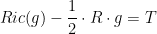
Coming back to Physics, Einstein’s General Relativity says that our universe is modeled by where is the space-time and is a Lorentzian metric. Here is a manifold of dimension 4 (where 3 dimensions corresponds to the space and 1 dimension corresponds to the time). However, in order to simplify our discussion, we’ll assume that (and is a product metric) for two reasons: this case is more easy to treat (since during most part of the discussion we can concentrate in the spatial part ) and a great part of the discussion can be generalized (with a little bit of technical work) to any . In this particular situation, Einstein’s equation relating Differential Geometry (curvature) and Physics (energy and momentum) is

where is the Ricci curvature of and is the stress-energy tensor. Unfortunately, due to the usual limitations of space and time (sorry for the implicit joke! :)), I’ll omit a detailed explanation of the terms appearing in this beautiful formula, but I hope that the reader will remember its main feature: it unifies the geometrical and physical aspects of space-time in a single equation. The relevant fact here is: the knowledge of the geometrical and physical aspects of the space-time are encoded by the metrics satisfying Einstein’s equation (for instance, the ‘straight lines’ of the metric geodesics are all possible trajectories in view of the minimal action principle, etc.)

In any case, once we arrived at Einstein’s equation, it is natural to ask about the existence of solutions. The first solution was discovered by K. Schwarzchild in 1916: it is the metric

on 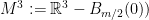, where is a real parameter and is the standard Euclidean metric on . Physically speaking, this solution models a famous entity called black hole with a mass placed at the origin . An interesting property of these black holes is the fact that the 2-dimensional sphere of radius works as an event horizon: any object (e.g., light) entering the ball can’t escape back to (actually, after entering the event horizon, they are attracted towards the origin).

A nice feature of the Schwarzschild’s solution is the natural identification of the real parameter with the mass of the black hole: in fact, the deviation of geodesics (i.e., curvature) increases proportionally to . Of course, this leads to the following natural problem in General Relativity: can we define a ‘good’ notion of mass of arbitrary space-times?

ADM mass in General Relativity. In general, the definition of mass in General Relativity (i.e., a natural notion which is invariant under change of coordinates [inertial referentials]) is a delicate issue. Nowadays, as we are going to see, one has such a notion only for a point or the entire Universe, but we don’t have a consensus (besides the several recent efforts) about a natural notion of a fixed non-trivial part of the Universe (i.e., a ”local mass”).

In any case, since we have a good notion of mass in the case of Schwarzschild black holes (namely, the parameter ), it is clear that any natural notion of mass should coincide with in Schwarzschild case. On the other hand, in order to introduce a definition of mass, we’ll make the physically reasonable hypothesis (based on the accepted theory that the entire Universe started with the Big-Bang, etc.) that the whole mass of the Universe (or more precisely massive objects) are confined to a bounded (i.e., compact) region, so that the gravitational effects tend to decay at infinity. Technically speaking, we are assuming that the metric is asymptotically flat (i.e., we are supposing that there is a compact set such that is diffeomorphic to and tends to the Euclidean metric [at a certain rate] at infinity).

Under these assumptions, the physicists R. Arnowitt, S. Deser and C. Misner introduced (in 1960) the following definition of mass (called ADM mass in their honor)

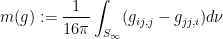
inspired by variational arguments with the action functional of Einstein-Hilbert . Here, is the ”sphere at infinity” (i.e., the previous integral should be interpreted as a limit), is the area element of , is the metric written in geodesic coordinates, are the derivates of (while is the scalar curvature and is the volume element).

Of course, this is a good definition of mass in the sense that the Australian mathematician R. Bartnik proved that the ADM mass is independent of the choice of coordinates (i.e., inertial referentials) and, after a straightforward calculation, one can show that in the case of Schwarzschild’s black holes.

One of the central theorems about the ADM mass (in General Relativity) is:

Theorem 1 (Positive mass theorem) Let be an asymptotically flat Riemannian manifold of scalar curvature (at every point). Then, . Furthermore, if and only if and (i.e., the ADM mass is zero exactly for the vacuum space-time).

Remark 1 Of course, the term can have any sign (usually it has negative sign when the ”potential” energy surpasses the ”kinetic” energy) so that the positivity of the ADM mass is very far from obvious. On the other hand, the previous theorem says that when the local density of energy (measured by the scalar curvature) is non-negative everywhere (i.e., ).

The first proof of this theorem was given by R. Schoen and S.T. Yau in 1979 using variational methods based on the geometry of minimal surfaces. Therefore, this permits to say that the Mathematical tools helped the understanding of the notion of mass in General Relativity (Physics). However, since the proof of this beautiful result is beyond the scope of this post, we’ll pass to the next topic: how the Physics helps the advance of important Mathematical problems.

–Physics helping Mathematics–

Momentarily, we’ll apparently change the focus of our discussion in order to discuss the famous Yamabe problem. In simple terms, Yamabe problem concerns the existence of very ”round” metric in a given Riemannian manifold. More precisely, given a compact boundaryless Riemannian manifold of dimension , we search for a metric conformal to (i.e., where is a positive function) whose scalar curvature is constant. This problem was coined ‘Yamabe problem’ because H. Yamabe considered this question (as a preliminary step of a program to attack Poincare’s conjecture [whose complete solution was given by G. Perelman pursuing different techniques]) and he claimed in 1960 to have positively solved the problem, although, as it was pointed out by the Australian mathematician N. Trudinger, Yamabe’s solution was incorrect.

Despite a crucial error in his solution, Yamabe introduced a nice idea to attack the problem, namely, he observed that the equation is equivalent to solving a certain Partial Differential Equation (PDE) in terms of . More precisely, after changing the factor by (the exponent is chosen to get the simplest equation possible), one can perform some computations to see that is equivalent to

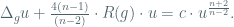
This PDE belongs to the well-known class of (non-linear) elliptic PDEs. At this point, Yamabe made his mistake: he believed that the existence of solutions of this PDE was a direct consequence of the theory of elliptic PDEs. However, this geometrically motivated elliptic PDE interestingly lies at the frontier of the theory of elliptic PDE (in other words, it is a critical PDE). More precisely, if the exponent of nonlinear term of the right-hand side of the equation were any number strictly less than , the usual (variational) methods of elliptic PDEs provide the desired solutions. But, since the exponent is exactly , we should work more. On the other hand, although the variational methods don’t solve directly the equation, it provides a simple criterion for the solvability of this PDE: it suffices to show that where

is the so-called Yamabe quocient of (and is the canonical sphere with the round metric of constant curvature ). Therefore, this reduces the Yamabe problem to the following problem: show that for any not globally conformal to .

Remark 2 Since is conformal to the standard Euclidean space by stereographic projection, we call conformally flat any manifold globally conformal to . In this notation, Yamabe problem is reduced to prove that non-conformally flat implies .

The case of and is not locally conformally flat (i.e., there is some region of where there are no conformal deformations of equal to the Euclidean metric) was treated by T. Aubin using adequate (depending on the Weyl tensor) local cut-offs of the functions

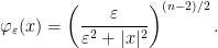
These functions are naturally associated to the problem because they realize the infimum of the expression defining . After a long series of computations, Aubin was able to show that in this situation, so that the Yamabe problem can be solved in the corresponding cases.

Therefore, this leaves the cases or locally conformally flat (but not globally conformally flat) open. Here, Richard Schoen had a brilliant idea: instead of performing local cut-offs of directly, he decided to glue these functions with certain Green functions of the Yamabe PDE (here is a term whose behaviour is equal to up to second order). After a long calculation, R. Schoen showed that

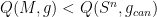
Hence, Yamabe problem can be positively solved in the remaining case once we can show that . Exactly at this moment, the Physics (General Relativity) comes to our rescue (another brilliant idea of Schoen): using the (properties of the) Green function (or more precisely its power ) as a conformal factor of , we can define a metric such that is asymptotically flat and . Thus, the positive mass theorem can be applied to conclude that (in fact, can’t happen since implies that is Euclidean, i.e., is globally conformally flat).

Now, after some more or less direct computations, R. Schoen shows an almost magical fact , so that the Yamabe problem is solved! In other words, the crucial point of the final part of Schoen’s argument is the use of the concept of ADM mass (Physics) to solve Yamabe problem (Mathematics).

Before closing the post, let me take the opportunity to say that, of course, this is not the end of the history of the fruitful (and unreasonably effective) interaction between Mathematics and Physics. In fact, some of examples of successful mutual feed-back are, for instance, Quantum Mechanics and Operator Algebra, Yangs-Mills theory and Donaldson construction of exotic structures of , String Theory and calculation of rational points of algebraic varieties in Enumerative Geometry. In any case, I hope you enjoyed this post! See you!