Romain Dujardin’s Bourbaki seminar talk 2018

Posted by: matheuscmss | January 3, 2019

Romain Dujardin’s Bourbaki seminar talk 2018

Last October, Romain Dujardin gave a nice talk at Bourbaki seminar about the equidistribution of Fekete points, pluripotential theory and the works of Robert Berman, Sébastien Boucksoum and David Witt Nyström(including this article here). The video of Dujardin’s talk (in French) is available here and the corresponding lecture notes (also in French) are available here.

In the sequel, I will transcript my notes for Dujardin’s talk (while referring to his text for all omitted details). In particular, we will follow his path, that is, we will describe how a question related to polynomial interpolation was solved by complex geometry methods, but we will not discuss the relationship of the material below with point processes.

Remark 1 As usual, any errors/mistakes in this post are my sole responsibility.

1. Polynomial interpolation and logarithmic potential theory in one complex variable

1.1. Polynomial interpolation

Let ${\mathcal{P}_k(\mathbb{C})}$ be the vector space of polynomials of degree ${\leq k}$ in one complex variable. By definition, ${\dim\mathcal{P}_k(\mathbb{C})=k+1}$ .

The classical polynomial interpolation problem can be stated as follows: given ${k+1}$ points ${z_0,\dots, z_{k+1}}$ on ${\mathbb{C}}$ , can we find a polynomial with prescribed values at ${z_j}$ ‘s? In other terms, can we invert the evaluation map ${ev(z_0,\dots,z_k):\mathcal{P}_k(\mathbb{C})\rightarrow \mathbb{C}^{k+1}}$ , ${P\mapsto (P(z_0),\dots, P(z_k))}$ ?

The solution to this old question is well-known: in particular, the problem can be explicitly solved (whenever the points are distinct).

What about the effectiveness and/or numerical stability of these solutions? It is also well-known that they might be “unstable” in many aspects: for instance, the inverse of ${ev(z_0,\dots, z_k)}$ starts to behave badly when some of the points ${z_0,\dots, z_k}$ get close together, a small error on the values ${P(z_0),\dots, P(z_k)}$ might lead to huge errors in the polynomial ${P}$ , Runge’s phenomenon shows that certain interpolations about equidistant point in ${[-1,1]}$ are highly oscillating, etc.

This motivates the following question: are there “optimal” choices for the points (leading to “minimal instabilities” in the solution of the interpolation problem)?

This vague question can be formalized in several ways. For instance, the interpolation problem turns out to be a linear algebra question asking to invert an appropriate Vandermonde matrix ${V(z_0,\dots, z_k)}$ and, a fortiori, the calculations will eventually oblige us to divide by an adequate determinant ${\det V(z_0,\dots, z_k)}$ . Hence, if we denote by ${e_i(z)=z^i}$ , ${i=0, \dots, k}$ , the base of monomials of ${\mathcal{P}_k(\mathbb{C})}$ , then we can say that an optimal configuration maximizes the modulus of Vandermonde’s determinant

$\displaystyle \det M(z_0,\dots, z_k) = \det(e_i(z_j))_{0\leq i, j\leq k} = \prod\limits_{0\leq i<j\leq k} (z_j-z_i).$

Of course, this optimization problem has a trivial solution if we do not impose constraints on ${z_0,\dots, z_k}$ . For this reason, we shall fix some compact subset ${K\subset \mathbb{C}}$ and we will assume that ${z_0,\dots, z_k\in K}$ .

Definition 1 A Fekete configuration ${(z_0,\dots,z_k)\in K^{k+1}}$ is a maximum of

$\displaystyle K^{k+1}\ni(w_0,\dots, w_k)\mapsto \prod\limits_{0\leq i<j\leq k} |w_j-w_i|$

Definition 2 The ${(k+1)}$ -diameter of ${K}$ is

$\displaystyle d_{k+1}(K) := \prod\limits_{0\leq i<j\leq k} |z_j-z_i|^{2/k(k+1)}$

where ${(z_0,\dots, z_k)}$ is a Fekete configuration.

It is not hard to see that ${d_{k+1}(K)\leq d_k(K)}$ , i.e., ${d_k(K)}$ is a decreasing sequence.

Definition 3 ${d_{\infty}(K)=\lim\limits_{k\rightarrow\infty} d_k(K)}$ is the transfinite diameter.

The transfinite diameter is related to the logarithmic potential of ${K}$ .

1.2. Logarithmic potential

In the one-dimensional setting, the equidistribution of Fekete configurations towards an equilibrium measure was established by Fekete and Szegö.

Theorem 4 (Fekete, Szegö) If ${d_{\infty}(K)>0}$ and ${F_k}$ is a sequence of Fekete configurations, then the sequence of probability measures

$\displaystyle \frac{1}{k+1}\sum\limits_{z\in F_k} \delta_z =:\frac{1}{k+1}[F_k]$

converges in the weak-* topology to the so-called equilibrium measure ${\mu_K}$ of ${K}$ .

Proof: Let us introduce the following “continuous” version of Fekete configurations. Given a measure ${\mu}$ on ${K}$ , its “energy” is

$\displaystyle I(\mu) := \int\log|z-w| \, d\mu(z) \, d\mu(w),$

so that if we forget about the “diagonal terms” ${\log|z_i-z_i|}$ , then ${I([F_k]) = \log d_{k+1}(K)}$ . Recall that the capacity of ${K}$ is ${\textrm{cap}(K)=\exp(V(K))}$ where ${V(K) = \sup \{I(\mu): \mu\in\mathcal{M}(K)\}}$ (and ${\mathcal{M}(K)}$ stands for the space of probability measures on ${K}$ ).

Theorem 5 (Frostman) Either ${K}$ is polar, i.e., ${I(\mu)=-\infty}$ for all ${\mu\in\mathcal{M}(K)}$ or there is an unique ${\mu_K\in\mathcal{M}(K)}$ with ${I(\mu_K)=V(K)}$ .

We are not going to prove this result here. Nevertheless, let us mention that an important ingredient in the proof of Frostman’s theorem is the logarithmic potential ${u_{\mu}(z)=\int\log|z-w|\,d\mu(w)}$ associated to ${\mu\in\mathcal{M}(K)}$ : it is a subharmonic function whose (distributional) Laplacian is ${\Delta u_{\mu} = 2\pi\mu}$ . A key feature of the logarithmic potential is the fact that if ${I(\mu) = V(K)}$ , then ${u_{\mu}(z)=V(K)}$ for ${\mu}$ -almost every ${z}$ : observe that this allows to conclude the uniqueness of ${\mu_K}$ because it would follow from ${I(\mu)=V(K)=I(\nu)}$ that ${u_{\mu}-u_{\nu}}$ is harmonic, “basically” zero on ${K}$ , and ${u_{\mu}-u_{\nu} = O(1)}$ near infinity.

Anyhow, it is not hard to deduce the equidistribution of Fekete configurations towards ${\mu_K}$ from Frostman’s theorem. Indeed, let ${\mu_k}$ be ${\frac{1}{k+1}[F_k]}$ and consider the modified energy ${\widetilde{I}(\mu_k) = \int_{z\neq w} \log|z-k|\,d\mu_k(z)\,d\mu_k(w) = \frac{k+1}{k}\log\delta_{k+1}(K)}$ . A straighforward calculation (cf. the proof of Théorème 1.1 in Dujardin’s text) reveals that if ${\mu_{k_j}}$ is a converging subsequence, say ${\mu_{k_j}\rightarrow\nu}$ , then ${I(\nu)\geq \log d_{\infty}(K) \geq V(K)}$ . $\Box$

1.3. Two remarks

The capacity of ${K}$ admits several equivalent definitions: for instance, the quantities

$\displaystyle \tau_k(K)=\inf\{\|P\|_K:=\sup\limits_{z\in K}|P(z)|: P \textrm{ is a monic polynomial of degree }\leq k\}$

form a submultiplicative sequence (i.e., ${\tau_{k+l}(K)\leq\tau_k(K)\tau_l(K)}$ ) and the so-called Chebyshev constant

$\displaystyle \tau_{\infty}(K) := \lim\limits_{n\rightarrow\infty}\tau_n(K)^{1/n}$

coincides with ${\textrm{cap}(K)}$ . In other terms, the capacity of ${K}$ is the limit of certain geometrical quantities ${\tau_k(K)}$ associated to a natural norm ${\|.\|_K}$ on the spaces of polynomials ${\mathcal{P}_k(\mathbb{C})}$ .

Also, it is interesting to consider the maximization problem for weighted versions

$\displaystyle I_Q(\mu) = I(\mu)+\int Q\,d\mu$

of the energy ${I(\mu)}$ of measures.

As it turns out, these ideas play a role in higher dimensional context discussed below.

2. Pluripotential theory on ${\mathbb{C}^n}$

Denote by ${\mathcal{P}_k(\mathbb{C}^n)}$ the space of polynomials of degree ${\leq k}$ on ${n}$ complex variables: it is a vector space of dimension ${\binom{n+k}{k}:=N_k\sim k^n/n!}$ as ${k\rightarrow \infty}$ .

Let ${K}$ be a compact subset of ${\mathbb{C}^n}$ and consider ${z_1,\dots, z_{N_k}\in K}$ . Similarly to the case ${n=1}$ , the interpolation problem of inverting the evaluation map ${\mathcal{P}_k(\mathbb{C}^n)\ni P\mapsto (P(z_1),\dots, P(z_{N_k}))\in\mathbb{C}^{N_k}}$ involves the computation of the determinant ${\det(e_i(z_j))}$ where ${(e_i)}$ is the base of monomials. Once again, we say that a collection ${(z_1,\dots, z_{N_k})}$ of ${N_k}$ points in ${K}$ maximizing the quantity ${|\det(e_i(z_j))|}$ is a Fekete configuration and the transfinite diameter of ${K}$ is ${d_{\infty}(K)=\limsup\limits_{k\rightarrow\infty} d_k(K)}$ where

$\displaystyle d_k(K) = \max\limits_{(z_1,\dots, z_{N_k})\in K^{N_k}}|\det(e_i(z_j))|^{1/kN_k}$

is the ${k}$ –diameter of ${K}$ .

Given the discussion of the previous section, it is natural to ask the following questions: do Fekete configurations equidistribute? what about the relation of the transfinite diameter and pluripotential theory?

A first difficulty in solving these questions comes from the fact that it is not easy to produce a “continuous” version of Fekete configurations via a natural concept of energy of measures having all properties of the quantity ${I(\mu)}$ in the case ${n=1}$ .

A second difficulty towards the questions above is the following: besides the issues coming from pairs of points which are too close together, our new interpolation problem has new sources of instability such as the case of a configuration of points lying in an algebraic curve. In particular, this hints that some techniques coming from complex geometry will help us here.

The next result provides an answer (comparable to Frostman’s theorem above) to the second question:

Theorem 6 (Zaharjuta (1975)) The limit of ${(d_k(K))_{k\in\mathbb{N}}}$ exists. Moreover, if ${K}$ is not pluripolar, then ${d_{\infty}(K)>0}$ .

Here, we recall that a pluripolar set is defined in the context of pluripotential theory as follows. First, a function ${u:\Omega\rightarrow[-\infty,+\infty)}$ on a open subset ${\Omega\subset\mathbb{C}^n}$ is called plurisubharmonic (psh) whenever ${u}$ is upper semicontinuous (usc) and ${u|_C}$ is subharmonic for any ${C\subset\Omega}$ holomorphic curve. Equivalently, if ${u\not\equiv-\infty}$ , then ${u}$ is psh when ${u}$ is usc and the matrix of distributions ${\left(\frac{\partial^2 u}{\partial z_j\partial\overline{z_k}}\right)}$ is positive-definite Hermitian, i.e., ${dd^cu:=\frac{i}{\pi}\sum\frac{\partial^2 u}{\partial z_j\partial \overline{z_k}} dz_j\wedge d\overline{z_k}\geq 0}$ . Next, ${E}$ is pluripolar whenever ${E\subset \{u=-\infty\}}$ where ${u\not\equiv-\infty}$ is a psh function.

An important fact in pluripotential theory is that the positive currents ${dd^c u}$ can be multiplied: if ${u_1,\dots, u_m}$ are bounded psh functions, then the exterior product ${dd^c u_1\wedge\dots\wedge dd^c u_m}$ can be defined as a current. In particular, we can define the Monge-Ampère operator ${MA(u)=(dd^c u)^n = \frac{n!}{\pi^n}\det\left(\frac{\partial^2 u}{\partial z_j\partial\overline{z_k}}\right)idz_1\wedge d\overline{z_1}\wedge\dots\wedge i dz_n\wedge d\overline{z_n}}$ on the space of bounded psh functions.

Note that ${MA(u)}$ is a positive current of maximal degree, i.e., a positive measure. This allows us to define a candidate for the equilibrium measure in higher dimensions in the following way.

Let

$\displaystyle \mathcal{L} = \{u \textrm{ psh on } \mathbb{C}^n \textrm{ with } u(z)\leq \log|z|+O(1) \textrm{ as }z\rightarrow\infty\}$

be the so-called Lelong class of psh functions. Given a compact subset ${K\subset\mathbb{C}^n}$ , let

$\displaystyle V_K(z) = \sup\{u(z): u\in\mathcal{L}, u|_K\leq 0\}.$

Observe that ${V_K(z)}$ is a natural object: for instance, it differs only by an additive constant from the logarithmic potential of the equilibrium measure of ${K}$ when ${n=1}$ . Indeed, this follows from the key property of the logarithmic potential (“ ${I(\mu)=V(K)}$ implies ${u_{\mu}(z)=V(K)}$ for ${\mu}$ -almost every ${z}$ ”) mentioned earlier and the fact that ${V_K}$ is a subharmonic function which essentially vanishes on ${K}$ .

In general, ${V_K(z)}$ is not psh. So, let us consider the psh function given by its usc regularization ${V_K^*(z):=\inf\{u(z): u \textrm{ usc, } u\geq V_K\}}$ . Note that ${V_K^*\geq V_K\geq 0}$ , so that we can define the equilibrium measure of ${K}$ as

$\displaystyle \mu_K:=(d d^c V_K^*)^n.$

It is worth to point out that ${V_K}$ can be recovered from the study of polynomials (in a similar way to our discussion of the Chebyshev constant in the previous section). More concretely, we have ${\frac{1}{k}\log |P|\in\mathcal{L}}$ for all ${P\in\mathcal{P}_k(\mathbb{C}^n)}$ and a result of Siciak ensures that

$\displaystyle V_K(z)=\sup\left\{\frac{1}{k}\log |P(z)|: k\in\mathbb{N}, P\in\mathcal{P}_k(\mathbb{C}^n), P\leq 1 \textrm{ on } K\right\}$

Finally, note that this discussion admits a weighted version where the usual Euclidean norm ${|.|}$ on ${\mathbb{C}^n}$ is replaced by ${|.| \exp(-Q)}$ , the determinant ${|\det (e_i(z_j))|}$ is replaced by ${|\det (e_i(z_j))| \exp(-Q(z_1))\dots \exp(-Q(z_{N_k}))}$ , etc.

3. Bernstein–Markov property

Let ${\mu}$ be a probability measure on ${K}$ giving zero mass to all pluripolar subsets. Since algebraic subvarieties are pluripolar (because they are included in the locus ${\log|P|=-\infty}$ of some polynomial ${P}$ ), we have that ${\mu}$ gives no weight to algebraic subvarieties. Hence, a polynomial ${P}$ with ${\|P\|_{L^2(\mu)} = 0}$ must vanish, i.e., ${P\equiv 0}$ .

It follows that ${\|.\|_{L^2(\mu)}}$ is equivalent to the uniform norm ${\|.\|_K}$ on the finite-dimensional vector spaces ${\mathcal{P}_k(\mathbb{C}^n)}$ , i.e., there is a (best) constant ${1\leq M_k(\mu)<\infty}$ such that

$\displaystyle \|P\|_{L^2(\mu)}\leq \|P\|_K\leq M_k(\mu)\|P\|_{L^2(\mu)}$

for all ${P\in\mathcal{P}_k(\mathbb{C}^n)}$ .

Definition 7 We say that ${\mu}$ has the Bernstein–Markov property if ${\lim\limits_{k\rightarrow\infty} M_k(\mu)^{1/k}=1}$ .

The following result ensures that one can “always” work with measures enjoying the Bernstein–Markov property:

Theorem 8 (Bloom–Levenberg) Every non-pluripolar compact subset ${K\subset \mathbb{C}^n}$ supports a probability measure with the Bernstein–Markov property.

Moreover, if ${K=\overline{\Omega}}$ where ${\Omega}$ is an open subset of ${\mathbb{C}^n}$ with smooth boundary, then the equilibrium measure ${\mu_K}$ has the Bernstein–Markov property (see this paper here):

Theorem 9 (Siciak) If ${K}$ is regular (i.e., ${V_K=V_K^*}$ is continuous), then ${\mu_K}$ has the Bernstein–Markov property.

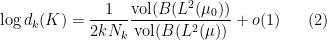
The Bernstein–Markov property is useful because it allows to interpret the transfinite diameter as the growth rate of certain volumes in the spaces of polynomials.

More concretely, let ${K}$ be a non-pluripolar set and ${\mu\in\mathcal{M}(K)}$ a probability measure with the Bernstein–Markov property.

Lemma 10 One has

$\displaystyle \int |\det(e_i(x_j))|^2\,d\mu(x_1)\dots d\mu(x_{N_k}) \leq d_k(K)^{2kN_k}\leq \widetilde{M}_k\int |\det(e_i(x_j))|^2\,d\mu(x_1)\dots d\mu(x_{N_k})$

with ${\lim\limits_{k\rightarrow\infty}\widetilde{M}_k^{1/kN_k}=1}$ .

Lemma 11 One has

$\displaystyle \int |\det(e_i(x_j))|^2\,d\mu(x_1)\dots d\mu(x_{N_k}) = N_k! \det(\langle e_i, e_j \rangle_{L^2(\mu)})$

Since the volumes of the unit balls of a vector space ${V}$ equipped with two Hermitian structures ${\langle.,.\rangle_1}$ and ${\langle.,.\rangle_2}$ are given by a Gram determinant, i.e.,

$\displaystyle \frac{\textrm{vol}(B_{\langle.,.\rangle_1}(0,1)}{\textrm{vol}(B_{\langle.,.\rangle_2}(0,1)} = \det(\langle e_i, e_j\rangle_1) \ \ \ \ \ (1)$

where ${(e_i)}$ is an orthonormal basis with respect to ${\langle.,.\rangle_2}$ , one gets from this fact and the previous two lemmas (whose [elementary] proofs are omitted) that

$\displaystyle \log d_k(K) = \frac{1}{2kN_k}\frac{\textrm{vol}(B(L^2(\mu_0))}{\textrm{vol}(B(L^2(\mu))}+o(1) \ \ \ \ \ (2)$

where ${\mu_0}$ is the Haar measure on the torus ${(\partial\mathbb{D})^n}$ and ${B(L^2(.))}$ is the unit ball of ${\mathcal{P}_k(\mathbb{C}^n)}$ with respect to the Hermitian structure ${L^2(.)}$ . (Here, it is natural to introduce ${\mu_0}$ because the base ${(e_i)}$ of monomials of ${\mathcal{P}_k(\mathbb{C}^n)}$ is orthonormal with respect to ${L^2(\mu_0)}$ .)

In summary, we saw that the transfinite volume ${d_{\infty}(K)}$ is related to the quotients of volumes of unit balls in the spaces of polynomials. In the last part of this post, we will investigate the problem of understanding quotients of volumes of unit balls in the more general setting of sections of positive vector bundles over complex manifolds.

4. Global pluripotential theory

Let ${X}$ be a compact complex manifold of dimension ${n}$ . Suppose that ${L\rightarrow X}$ is an ample line bundle, i.e., there is a smooth metric ${h}$ which is strictly psh (in the sense that any local trivialization ${s}$ of ${L}$ has the property that ${|s(x)|_h:=\exp(-\phi(x))}$ with ${d d^c\phi > 0}$ ).

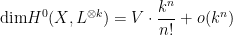
By the asymptotic Riemann-Roch theorem, the dimensions of the spaces ${H^0(X,L^{\otimes k})}$ of sections of the ${k}$ th tensor power ${L^{\otimes k}}$ of ${L}$ verify

$\displaystyle \textrm{dim}H^0(X,L^{\otimes k}) = V\cdot \frac{k^n}{n!}+o(k^n)$

as ${k\rightarrow\infty}$ , where ${V}$ is the volume of ${L}$ .

Example 1 For the line bundle ${L=\mathcal{O}(1)}$ over the complex projective space ${X=\mathbb{P}^n}$ , the space ${H^0(X,L^{\otimes k})}$ identifies with ${\mathcal{P}_k(\mathbb{C}^n)}$ (in a given chart of ${X}$ )

Let us fix ${h_0}$ a reference metric whose curvature form is denoted by ${\omega}$ . Note that all metrics on ${X}$ have the form ${h=h_0\exp(-\phi)}$ where ${\phi}$ is a function. We say ${h}$ is semi-positive (i.e., ${h\geq 0}$ ) whenever ${\phi \omega}$ is psh in the sense that ${dd^c\phi+\omega\geq 0}$ .

Given a smooth positive measure ${\mu}$ on ${X}$ and a metric ${h}$ on ${L}$ , one has a natural ${L^2}$ -structure ${\|.\|_{L^2}}$ on ${H^0(X,L^{\otimes k})}$ , namely

$\displaystyle s\mapsto \left(\int |s(x)|_{h_k}^2 d\mu(x)\right)^{1/2}$

where ${h_k}$ stands for the metric induced on ${L^{\otimes k}}$ by ${h}$ .

Theorem 12 (Berman–Boucksoum) Let ${\mu_1}$ , ${\mu_2}$ be two smooth positive measures and ${h_1}$ , ${h_2}$ two metrics on ${L}$ . Then,

$\displaystyle \frac{1}{2kN_k}\frac{\textrm{vol}(B_{H^0(X,L^{\otimes k})}(L^2(\mu_1, h_1)))}{\textrm{vol}(B_{H^0(X,L^{\otimes k})}(L^2(\mu_2, h_2)))}\longrightarrow\mathcal{E}(h_1)-\mathcal{E}(h_2) \quad \textrm{as } k\rightarrow\infty,$

where ${\mathcal{E}(h):=\frac{1}{(n+1) \textrm{vol}(h)} \sum\limits_{j=0}^n \int_X \phi(\omega+dd^c\phi)^j\wedge\omega^{n-j}}$ is the Monge-Ampère energy of ${h=h_0\exp(-\phi)}$ .

(Here, we insist on the quotients of volumes because the volumes are well-defined only up to a multiplicative constant.)

The Monge-Ampère energy is an interesting functional playing the role of a primitive of the Monge-Ampère operator ${MA(\phi):=\frac{1}{\textrm{vol}(L)}(\omega+dd^c\phi)^n}$ in the sense that

$\displaystyle \frac{d}{dt}\mathcal{E}(\phi+tv)|_{t=0}=\int v \cdot MA(\phi)$

The idea of proof of Berman–Boucksoum theorem above goes along the following lines (cf. this article here for more details). We write ${\mathcal{E}(h_1)-\mathcal{E}(h_2) = \int (\phi_1-\phi_2)\cdot MA(\phi_t)}$ where ${\phi_t}$ is a path connecting ${\phi_1}$ and ${\phi_2}$ . The quotient of volumes in the left-hand side is a Gramm determinant (similar to (1)) with respect to an appropriate choice of basis of sections of ${H^0(X,L^{\otimes k})}$ and its derivative is the so-called Bergman kernel. In particular, the desired result comes from a comparison between Monge-Ampère operators and Bergman kernels.

For some applications of this result (e.g., to the study of Fekete configurations), it is important to improve this theorem to the case of general measures ${\mu_1}$ and ${\mu_2}$ . As it turns out, this is done by considering the quotients of volumes with respect to ${L^{\infty}}$ norms on ${H^0(X,L^{\otimes k})}$ induced by the metrics and the Monge-Ampère energies of certain functions ${P_K^*(\phi)}$ playing the analog role of the functions ${V_K}$ introduced above in the context of compact subset ${K\subset\mathbb{C}^n}$ .

Anyhow, let us close this post by explaining how this technology can be used to get the equidistribution of Fekete points in higher dimensional settings.

5. Equidistribution of Fekete configurations

We saw that the transfinite diameter is related to the quotient of two volumes (cf. (2)). In order to exploit this fact, we need the following result of Berman–Boucksoum.

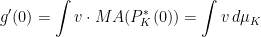
Theorem 13 (Berman–Boucksoum) The Monge-Ampère energy ${\mathcal{E}(P_K^*\phi)}$ is differentiable with respect to ${\phi}$ , namely

$\displaystyle \frac{d}{dt}\mathcal{E}(P_K^*(\phi+tv))|_{t=0}=\int v \cdot MA(P_K^*(\phi))$

Remark 2 The Monge-Ampère measure ${MA(P_K^*(\phi))}$ is the candidate to the equilibrium measure.

Besides the previous theorem, we also need a technical fact about concave functions of the real line:

Lemma 14 Let ${f_k}$ be a sequence of (differentiable) concave functions defined in a neighborhood ${U}$ of ${0\in\mathbb{R}}$ . If ${g}$ is a (differentiable) concave function on ${U}$ such that

$\displaystyle \liminf\limits_{k\rightarrow\infty} f_k\geq g$

and

$\displaystyle \lim\limits_{k\rightarrow\infty} f_k(0)=g(0),$

then ${\lim\limits_{k\rightarrow\infty} f'_k(0)=g'(0)}$ .

At this point, the idea is to derive the equidistribution ${\frac{1}{N_k}[F_k]\rightarrow \mu_K}$ of Fekete configurations ${F_k}$ towards an equilibrium measure ${\mu_K}$ in higher dimensional settings from the previous lemma applied to the geometric functionals

$\displaystyle f_k(t) = -\frac{1}{2kN_k} \log\textrm{vol}(B_{\mathcal{P}_k(\mathbb{C}^n)}(L^2(\frac{1}{N_k}[F_k], e^{-t v})))$

and

$\displaystyle g(t) = \mathcal{E}(P_K^*(tv)$

because a straightforward calculation reveals that

$\displaystyle f_k'(0) = \frac{1}{N_k}\sum v(x_i)$

and Theorem 13 and (the generalization to arbitrary measures of) Theorem 12 yield

$\displaystyle g'(0)=\int v \cdot MA(P_K^*(0)) = \int v \, d\mu_K$

Remark 3 After the end of the talk, I asked Romain about speed of equidistribution of Fekete points and he pointed out to me that such results were recently obtained by T.-C. Dinh, X. Ma and V.-A. Nguyên.

Posted in expository, math.AG, Mathematics | Tags: Bernstein-Markov property, David Witt Nystrom, equidistribution, Fekete points, logarithmic potential, Monge-Ampere operator, pluripotential theory, plurisubharmonic function, polynomial interpolation, Robert Berman, Romain Dujardin, Sebastien Boucksoum, transfinite diameter

M	T	W	T	F	S	S
	1	2	3	4	5	6
7	8	9	10	11	12	13
14	15	16	17	18	19	20
21	22	23	24	25	26	27
28	29	30	31

	Adam on Breuillard-Sert’s joint…
	Adam on Breuillard-Sert’s joint…
	Writing a Hilbert C*… on ERT16: Compact extensions
	matheuscmss on Yoccoz book collection at…
	Jairo B. on Yoccoz book collection at…

Disquisitiones Mathematicae